Playing an item: how MakeSound() works

This page is for programmers who want to read, maintain or extend the code that turns a timed item into sound: real-time MIDI, a MIDI file, a Csound score, an event list, and the pianoroll that displays it. All of this is done by one function, MakeSound(), in the console's source file MakeSound.c. The page describes its algorithm step by step.

The code lives in three C files of the console (source/BP3/):

  • MakeSound.c contains MakeSound() and its subroutines;
  • Graphic.c contains PreparePianoroll(), which computes the layout of the pianoroll before the item is played;
  • -BP3.h defines the PianoRoll structure shared by these two files.

Comments of the form // note 12 have been placed in these files. Each one points to the numbered note of this page that explains the code below it. Searching for // note 12 finds every place that note 12 describes. Line numbers are not given because they change with every revision.

Where MakeSound() stands in the production of music

A grammar produces an item: a string of terminal symbols, notes, performance controls and polymetric structures such as {2, C4 D4 E4, F3 G3}. Playing this item takes four steps, all called from PlayBuffer1() in PlayThings.c:

  1. PolyMake() (Polymetric.c) expands the polymetric structure into a regular grid called the phase diagram.
  2. FillPhaseDiagram() places every sound-object, note and control on this grid, and SetTimeObjects() (TimeSet.c) computes the date at which each one starts and ends. Constraints such as overlapping, truncation, pivots and cyclic objects are resolved here.
  3. MakeSound() reads the list of timed objects and sends their events, in chronological order, to the selected outputs.
  4. DrawItem() draws the graph of sound-objects, if requested.

When MakeSound() starts, therefore, all decisions about when things happen have been taken. Its task is to merge the events of all objects into a single chronological stream, to compute the MIDI or Csound values of each event (key, velocity, channel, controls), and to keep track of which keys are sounding so that every NoteOn gets its NoteOff.

The data received by MakeSound()

The main input is the global table p_Instance. Each entry (*p_Instance)[k], for k = 2 to *p_kmax, is a sound-object instance: one occurrence of an object in the item. (Indices 0 and 1 are not used for instances.) Its main fields are:

  • object, called j in the code: what is played. Its value tells what kind of object it is: 
    • j == 0: no object. Terminal 0 is the prolongation _
    • j = 1: silence -
    • 1 < j < Jbol: a sound-object, whose prototype is defined in a -so file. Its events are in (*pp_MIDIcode)[j], a list of MIDI bytes, and possibly in (*pp_CsoundScore)[j], a list of Csound score lines.
    • Jbol ≤ j < 16384: a time pattern, which marks time but produces no sound.
    • j ≥ 16384: a simple note such as C4, whose MIDI key is j - 16384.
    • j < 0: an out-time object (written <<…>>), which has no duration. The code works with -j and sets outtime.
  • starttime, endtime: dates in milliseconds computed by SetTimeObjects().
  • truncbeg, truncend: durations cut at the beginning and at the end of the object, when constraints did not allow it to be played entirely.
  • alpha, beta: dilation ratios. alpha is the ratio between the duration of the object in the item and the duration of its prototype. beta is the ratio applied to the dates of its events. They are equal unless the object is cyclic: a cyclic object stretched by 3 keeps beta = 1 and repeats its periodical part instead (note 4).
  • nseq: the sequence (line of the phase diagram) on which the object is placed. Performance parameters are stored per sequence.
  • channel, velocity, transposition, scale, blockkey, instrument: the values of the performance controls (_chan(), _vel(), _transpose(), _scale(), _ins()…) in force when the object starts.
  • contparameters: the values of continuous parameters (pitchbend, volume, modulation, pressure, panoramic, and Csound parameters), with their start and end values and their mode: fixed, stepwise or continuous.
  • map0, map1, mapmode: key mapping (_keymap()), possibly varying from map0 to map1 during the object.

The other arguments of MakeSound() are tmin and tmax, the limits of the item in time, maxnsequences, the number of sequences, and imaxstreak and p_delta, which are only used to draw the background of the pianoroll.

Overview of the algorithm

Each instance is a stream of events ordered by date. MakeSound() merges these streams, together with the streams of messages generated by continuous controls, into one chronological stream. It does so without sorting the events: it keeps for each instance k the index (*p_inext)[k] of its next event and the date (*p_nextd)[k] of this event, and repeatedly:

  1. picks the instance whose next event comes first, at date t2;
  2. sends the events of this instance that are due at t2 (none of them can be later than the next event of another stream);
  3. saves the position reached in this instance, and goes back to step 1.

This is a k-way merge. Finding the next instance scans all instances, so the cost is proportional to the number of events times the number of instances. It does not require building and sorting a list of all events, and it allows an item to be played while it is computed in real time.

Four dates, all in milliseconds, drive this loop:

  • t0: the origin of the current performance on the output clock;
  • t1: the date of the current event, relative to t0;
  • t2: the date of the next event in any other stream, relative to t0;
  • t3: the date at which the current instance ends, minus its post-roll.

Every event is sent at date t0 + t1. The global Tcurr holds the same date in units of Time_res milliseconds. It is read by the MIDI driver, by scripts and by the functions that write files, so the code updates it whenever t1 changes.

The steps of MakeSound() are:

  1. Preparation: choose the outputs, allocate the working tables, scan the instances to find the first one and the first event of each (notes 1–4).
  2. Pianoroll: compute its limits in time and pitch, and draw its background (note 5).
  3. Outputs: open the Csound score and the MIDI file, tune the MIDI device (notes 6–7).
  4. Performance loop, repeated Nplay times: set the time origin (notes 8–10), then run the scheduler (notes 11–36).
  5. End of the item: release the keys still sounding, append the final silence, close the Csound score, free the memory (notes 37–40).

Notes 41 to 51 describe the subroutines.

Step 1 — Preparation

Note 1 — Choosing the outputs

The function returns at once if a performance is already running (SoundOn) or if the user has pressed PANIC. Without a trace path (--traceout), no graphics can be saved, so they are switched off.

Two local flags decide where the events go:

  • cswrite is TRUE if a Csound score is written. This happens when Csound output is selected and the item is not played in real time (or FileWriteMode is NOW), or when a MIDI file is converted to Csound. In the rest of the code, cswrite selects the Csound branch of every decision: no MIDI event is sent, and CscoreWrite() (CsoundScoreMake.c) writes score lines instead.
  • The global MIDIfileOn is TRUE if a MIDI file is written, under the same condition.

Real-time MIDI is rtMIDI, the event list is EventListOn, and the pianoroll is showpianoroll. The pianoroll is not drawn during a MIDI capture (ItemCapture) or when converting MIDI to Csound. If no output is selected, nothing is done. When several items are produced, ItemNumber counts them, and production stops after MaxItemsProduce items.

The pianoroll is drawn while the item is played, in the same pass: each note is drawn when its NoteOff is sent. It does not require a separate traversal of the events.

Note 2 — Working tables

All tables are Handles (see ConsoleMemory.c), allocated at the start and freed at the end (note 40).

  • Per instance (size MaxObjects):
    • p_inext: index of the next event to send; p_inext1: index of the first event, restored at each performance;
    • p_nextd: date of the next event; Infpos means that the instance is over;
    • p_onoff: TRUE once the instance has started (note 16);
    • p_silence: TRUE when the NoteOns of the instance must be silenced because its end is truncated (note 34);
    • p_istartperiod, p_iendperiod, p_periodgap, p_icycle: the periodical part of cyclic objects (notes 4 and 32).
  • Per MIDI channel and key (16 × 128): 
    • p_keychannel[ch][key]: the number of NoteOns of this key not yet followed by a NoteOff. Several objects can play the same key at the same time, so this is a counter, not a flag;
    • p_last_timeon[ch][key]: the date of the last NoteOn of this key, used to draw the note on the pianoroll and to detect NoteOns that are too close (note 28).
  • Per Csound instrument and key: p_keyinstrument[ins][key], the same counter as p_keychannel, used when cswrite is TRUE.
  • Per channel and continuous parameter: p_active, p_t2cont and p_seqcont describe the continuous controls being sent (note 19).
  • Per sequence:
    • pp_currentparams[nseq]: the performance parameters used by CscoreWrite() (note 17);
    • p_control[nseq]: the streams of continuous MIDI controls (note 19).
  • p_currmapped: the keys changed by key mapping, so that a NoteOff finds the key of its NoteOn (note 51).

Note 3 — Scanning the instances

A first loop over all instances prepares the scheduler. For each instance it:

  • finds the number of events of the object, im, with Find_im(). This is the number of MIDI bytes of the prototype, or the number of lines of its Csound score if that score is played (note 49). A time pattern has no events.
  • sets beta = alpha if the object is played less than twice and its prototype is not of fixed scale. Only a cyclic object keeps a beta different from alpha.
  • finds the first event of the object, (*p_inext1)[k]. The dates of events are obtained by adding the delays between consecutive events, multiplied by beta (EventDelay(), note 46).
  • finds the instance that starts first, kfirstinstance, at date t11, and the start date of the next one, t22. A negative pre-roll moves the start of an object earlier.

The scheduler starts with instance kfirstinstance, t1 = t11 and t2 = t22. As soon as this instance starts, t2 is computed again from all instances (note 16).

Note 4 — Cyclic objects

A sound-object prototype can be declared cyclic: when it must last longer than its prototype (alpha > 1), its events are not stretched; instead, the part that follows cyclicafter is repeated. GetPeriod() (SoundObjects2.c) returns cyclicafter, the date at which the periodical part starts, and objectperiod, its duration.

The scan stores:

  • (*p_istartperiod)[k]: the first event at or after cyclicafter;
  • (*p_iendperiod)[k]: the last event of the first cycle, extended to the following events that are simultaneous with it;
  • (*p_periodgap)[k]: the time between the start of a period and its first event, plus the time between its last event and the end of the cycle;
  • time_nextperiod_start: the date at which the second cycle starts.

For an object that is not cyclic, istartperiod remains -1. Note 32 explains how the scheduler uses these values.

Step 2 — The pianoroll (Graphic.c)

Note 5 — Limits in time and pitch

The pianoroll is an image in which each note is a horizontal bar: its position is its date, its height is its key. Before the first note can be drawn, the size of the image must be known. PreparePianoroll() computes it:

  • The end of the item, tmax, is the largest end date of all instances, increased by the post-roll of sound-objects and by the opposite of a negative pivot. The image covers Nplay repetitions of the item.
  • The range of keys, minkey to maxkey, includes the key of every simple note and the key of every NoteOn in the MIDI codes of sound-objects, after transposition, expansion and key mapping (note 51). For a sound-object whose Csound score is played, the pitch of each score line is converted to a key by CsoundPitchToKey(), according to the pitch format of its instrument: octave point pitch-class (OPPC), octave point decimal (OPD) or frequency in Hertz (CPS). The range is then widened to multiples of 6.
  • The image starts at date 0, or earlier if a pivot or a pre-roll creates negative dates. leftoffset is the x position of date tmin, topoffset the y position of the top of the note scale, and hrect the height of one key (3 pixels). The width is limited to 32000 pixels.

These values are returned in a PianoRoll structure (roll in MakeSound()), which is passed to every function that draws a note. If ShowGraphic is set, PreparePianoroll() also draws the background (DrawItemBackground()) and the note scale (DrawNoteScale()). The field noteoffset is the x position from which notes are drawn. It is set by MakeSound() for each performance (note 10).

Step 3 — Opening the outputs

Note 6 — Preparing the outputs

  • In real time, the clock of the driver is read. When improvising, the time taken to compute the item is recorded in MaxComputeTime if it is the longest so far.
  • If the diapason A4freq is not 440 Hz, TuneMIDIdevice() sends the A4 tuning to all channels of the MIDI device (note 44).
  • For Csound, PrepareCsFile() opens the score. For a MIDI file, PrepareMIDIFile() (MIDIfiles.c) writes its header. In both cases Nplay is set to 1: repetitions are only meaningful in real time.

Note 7 — Resetting the performance parameters

For each sequence, the Csound performance parameters are reset: no key is sounding (level[key] = 0), there is no transposition, and no parameter is active. paramsinstance, the instance whose parameters are currently stored for this sequence, is set to 0 (note 15). All streams of continuous controls are marked inactive (ibm = -1).

Step 4 — The performance loop

Note 8 — Repeating the item

The item is played Nplay times, or forever if SynchroSignal is PLAYFOREVER. Each repetition is called an occurrence. stop() (ConsoleMain.c) is called at the start of each occurrence and before each event: it checks whether the user has clicked STOP or PANIC in the interface, which creates a file in temp_bolprocessor/.

Note 9 — Resetting the instances, truncated beginnings

At the start of each occurrence, every instance is reset: its next event is its first event (p_inext1), it has not started (p_onoff FALSE), and its next date is its start date.

If the beginning of an instance is truncated (truncbeg > 0), the events before the truncation are not played. FirstEventAfterTruncation() (note 47) finds the first NoteOn at or after the truncation, and the time this_gap between them. Starting at a NoteOn avoids sending NoteOffs or controls of notes that were cut. The next date of the instance is then its start date plus this_gap.

All keys are released in the tables of note 2, all switches (pedals) are off, and no continuous control is active.

Note 10 — The time origin

t0 is the date, on the clock of the output, at which date 0 of the item will be played. It depends on the situation:

  • Normally, currenttime = Tcurr × Time_res, the current date of the output. In real time and in MIDI files, MIDIsetUpTime is added once, to give the MIDI device time to receive the first messages.
  • If the item is played as a continuous flow (CyclicPlay) and the driver is already late, the item starts at the current time of the driver.
  • When an item is played line by line in chunks, each chunk starts at the end of the previous one, ChunkEndTime.
  • If t1 is negative (an object starts before date 0 because of a pivot or a pre-roll), t0 is moved later by -t1, so that no event has a negative date.
  • When several items follow each other (improvisation, all items, chunks), t0 is the end of the previous item, LastTime. PianorollShift records this offset so that the pianoroll of each item starts at its own origin.

The pianoroll's noteoffset is set here: it is leftoffset, shifted back if all dates were shifted by -t1.

ChunkEndTime and, in real time, ExpectedEndTime are computed at the first occurrence. ExpectedEndTime is the date at which the item will end, displayed by the clock of produce.php.

For Csound, WriteCsoundTempo() writes the tempo statement at the start of the score (note 45).

Note 11 — The scheduler

The loop while(kcurrentinstance > 0) is the heart of MakeSound(). Each iteration works on one instance, kcurrentinstance:

  1. read the context of the instance (notes 12–15);
  2. if the instance has not started yet, start it: send its initial controls, script and switches (notes 16–20);
  3. send its events while t1 ≤ t2 and t1 ≤ t3 (notes 21–33);
  4. record where it stopped, or that it is over (note 34);
  5. send a message of a continuous control if one is due (note 35);
  6. find the next instance or control (note 36).

The loop ends when NextInstance() returns 0: no instance has an event left.

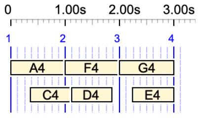
Here is an example with C4 {D4, E4 F4} at 60 beats per minute. Instance 2 is C4 (0–1000 ms), 3 is D4 (1000–2000), 4 is E4 (1000–1500), 5 is F4 (1500–2000). The next dates of the instances are 0, 1000, 1000 and 1500.

  1. Instance 2 starts, and t2 becomes 0, its own date. It sends NoteOn C4 at 0. Its next event, the NoteOff at 1000, is later than t2, so it is suspended with next date 1000.
  2. Instances 2, 3 and 4 now have the earliest date, 1000. The first one in the table is chosen: instance 2 sends NoteOff C4 at 1000 and is over.
  3. Instance 3 sends NoteOn D4 at 1000 and is suspended until 2000. Instance 4 sends NoteOn E4 at 1000 and is suspended until 1500.
  4. At 1500, instance 4 comes before instance 5: it sends NoteOff E4, then instance 5 sends NoteOn F4.
  5. At 2000, instance 3 sends NoteOff D4, then instance 5 sends NoteOff F4.

At equal dates, instances are taken in the order of the table, which is the order of the item. A note that ends is therefore released before the next note of the same sequence starts, as at step 4.

Note 12 — Context of the current instance

Each time the scheduler comes back to an instance, it reads its parameters: object j, scale, block key, channel (converted by ChannelConvert(), note 49), sequence nseq, dilation ratios. A negative j indicates an out-time object (see “The data received by MakeSound()”).

Note 13 — Number of events

The events of an instance are indexed by ievent, from 0 to im - 1:

  • for a sound-object whose MIDI codes are played, ievent is the index of a byte in (*pp_MIDIcode)[j]. A NoteOn takes three entries (status, key, velocity). Each entry has a time field, the delay in milliseconds since the previous entry, before dilation;
  • for a sound-object whose Csound score is played, ievent is the index of a line of the score, (*pp_CsoundScore)[j];
  • a simple note has im = 6: two “virtual” messages of three bytes, a NoteOn at ievent = 0 and a NoteOff at ievent = 3 (note 33).

The pre-roll and post-roll of the prototype (ObjectPreRoll(), ObjectPostRoll(), note 46), its cyclic period (note 4), and its strike again setting (note 28) are also read here.

Note 14 — End date and duration

The instance must stop at t3, its end date minus the post-roll of its prototype. objectstarttime is its start date minus the truncated part, and earlier by a negative pre-roll. objectduration = t3 - objectstarttime is used to spread continuous controls and key mappings over the object. A negative or unreasonably long duration (over 500 seconds) indicates an error in the time-setting. It is reported, and the duration is set to 0.

Note 15 — Restoring the Csound parameters of a resumed object

The Csound parameters (note 17) are stored per sequence, not per instance. If an object is interrupted by the start of another object on the same sequence, its parameters are replaced. When the scheduler comes back to the first object, its own parameters are therefore copied back with SetObjectParameters(). paramsinstance records which instance the parameters of the sequence belong to, so the copy is only made when it has changed. Example: in _volumecont _volume(30) a C4 … _volume(127), if sound-object a lasts longer than its time slot, its events after the start of C4 keep the volume variation of a.

Note 16 — Starting an instance

The first time the scheduler comes to an instance, (*p_onoff)[k] is FALSE. The instance is then started:

  • it is added to the event list if one is written (AddEventToList());
  • its MIDI channel is computed by MIDIchannel() (note 49);
  • unless it is out-time, SendInitialControls() sends its volume, panoramic, pitchbend, pressure and modulation on this channel if they have changed (note 42);
  • t2 is computed again, since the start of this instance may change which stream comes next (NextInstance() and NextControlDate(), note 48).

Note 17 — Csound parameters

The parameters of the instance (contparameters) are copied to those of its sequence (pp_currentparams[nseq]->params) by SetObjectParameters(). CscoreWrite() reads them to compute the parameter fields of each score line: for a continuous variation, it interpolates between startvalue and endvalue (or along a table of points) according to the date of the event within the object.

The table of a sequence is created with only the five MIDI parameters (IPANORAMIC + 1), and enlarged here to MaxParameters + IPANORAMIC + 1 entries, adding the parameters declared in the Csound instruments. The table of an instance always has this size, since SetObjectParams() (SetObjectFeatures.c) creates it that way. A different size is reported as an error.

SetObjectParameters() marks a parameter inactive in these cases, so that CscoreWrite() uses its default value:

  • volume or panoramic, when the prototype does not accept them;
  • an additional parameter without a value;
  • a continuous MIDI parameter set on another channel than the object's.

Note 18 — Scripts

An object can carry script commands, such as _script(wait for C3 channel 1) or _script(MIDI send Start). ExecuteScriptList() executes them in order when the object starts, through ExecScriptLine() (Script.c). A command can make the performance wait. The time spent waiting is added to LapWait, and WaitEndDate is shifted accordingly.

Note 19 — Continuous MIDI controls

A continuous variation of a MIDI parameter, such as _pitchbend(0) _pitchcont … _pitchbend(200), cannot be sent as a single message: it is sent as a stream of messages at regular intervals during the object. For each of the five MIDI parameters (pitchbend, volume, modulation, pressure, panoramic) whose mode is CONTINUOUS, a stream is set up in (*p_control)[nseq].param[index]:

  • starttime, duration: the start date and duration of the object;
  • startvalue, endvalue, and possibly a table of points point with imax entries;
  • channel: the channel on which the variation was set;
  • ibm: the number of messages, computed by Findibm() from the duration and the rate (messages per second) set for this parameter and channel in the settings; ib: the number of messages already sent.

Only one stream per channel and parameter can be active at a time. (*p_active[ch])[index] tells whether a stream is active, (*p_seqcont[ch])[index] on which sequence it is, and (*p_t2cont[ch])[index] the date of its next message. If a stream was still active on this channel (it may not have ended because of rounding), its last message is sent first. The new stream sends its first message at once, and the date of its next message may become the new t2.

When a Csound score line of the object is played (PlayCsoundLine()), these streams are skipped: Csound variations are handled by CscoreWrite() (note 17). The messages of the streams are sent by SendControl() (notes 35 and 50).

Note 20 — Switches and dilation ratio

Switches are the MIDI controllers 64 to 69, including the sustain pedal (64), set with _switchon() and _switchoff(). SendSwitches() (note 43) sends those that have changed when the object starts. The state of the switches of each channel is kept in currswitchstate[ch], one bit per switch.

If the prototype asks for it, SendDilationRatio() (note 44) sends the dilation ratio beta of the object to a MIDI controller. This allows a synthesizer to adapt the sound to the speed of the performance.

Note 21 — Sending the events of an instance

The inner loop sends the events of the current instance as long as:

  • t1 ≤ t2: no other stream has an event before this one;
  • t1 ≤ t3: the instance has not reached its end;
  • ievent < im: the instance has events left.

When two streams have events at the same date, the current instance goes first, which avoids switching between instances for simultaneous events. Each event is processed by notes 22 to 31, then t1 and ievent are advanced to the next event (notes 32 and 33).

Note 22 — End of a cyclic object

When a cyclic object reaches its end (t1 ≥ t3) and integer cycles are not forced, the last cycle is incomplete. If the last event of the object has been reached, all keys still sounding on its channel are released, and the loop moves on to the end-of-period test (note 32).

Before each event, howmuch is computed: the fraction of the object already played, from 0 to 1. Key mapping uses it to move progressively from map0 to map1 (note 51).

Note 23 — Csound score lines of a sound-object

If the prototype has a Csound score and a Csound score is written, the line ievent is passed to CscoreWrite() with its date t0 + t1 and the dilation ratio beta, which scales its duration. If the end of the object is truncated, cut_the_end is the part of this line that falls after the truncation, and its duration is shortened accordingly. No line is written while the object is silenced (note 34).

Note 24 — Decoding an event

Otherwise, the event is a MIDI message. Its status byte c0 is read:

  • for a sound-object, from its MIDI codes;
  • for a simple note or a time pattern, it is NoteOn if ievent == 0, else NoteOff.

MIDIchannel() separates the channel from the status byte (note 49). localchan is the channel on which the message is sent: the one in the MIDI code, the default channel of the prototype, or the channel of the object.

For a NoteOn or NoteOff, the key c1 and the velocity c2 follow. They are read from the next two bytes for a sound-object, or computed for a simple note: GoodKey(j) and velocity 127, which ClipVelocity() will scale. A time pattern produces nothing: its events are skipped.

Note 25 — Transposition and expansion

The key is transposed (_transpose()) and expanded (_keyxpand()) by TransposeAndExpand(). The order of these two operations depends on the order in which they were written in the item (transposefirst). GoodKey() brings the key of a simple note into the range 0–127 by octaves, with an error message.

Note 26 — NoteOff

A NoteOff, or a NoteOn with velocity 0, which MIDI treats as a NoteOff, is handled as follows:

  1. If key mapping changed the key of the matching NoteOn, RetrieveMappedKey() returns the mapped key (note 51).
  2. The counter p_keychannel[localchan][c1] is decreased. If it was already 0, the NoteOff is ignored: its NoteOn was merged with another one (note 28) or not played.
  3. The NoteOff is only sent when the counter reaches 0, i.e. when no other object is still holding this key. In Csound, every NoteOff is passed to CscoreWrite(), which finds the matching NoteOn and writes the score line with its duration. The counter p_keyinstrument of the instrument is decreased.
  4. In MIDI, SendNoteOffAndDraw() sends the NoteOff and draws the note on the pianoroll from its NoteOn date (note 41).

Note 27 — NoteOn: key mapping

If key mapping applies to this object (always for simple notes, according to the prototype for sound-objects), MapThisKey() gives the key to play (note 51). The pair (original key, played key) is stored by StoreMappedKey() after the NoteOn is sent, so that the NoteOff of the original key releases the played key. The counter of the key is then increased.

Note 28 — NoteOn: repeated keys

Two problems arise when a key is struck while it is already sounding:

  • MIDI cannot play the same key twice on the same channel. If the prototype (or the settings) asks to strike again (StrikeAgainOf(), note 46), a NoteOff is sent before the new NoteOn. Otherwise the NoteOn is not sent (strike = FALSE), and the key goes on sounding.
  • Two NoteOns of the same key very close in time are often an artefact of the polymetric structure, for example a note ending and the same note starting a few milliseconds later. If the key is still sounding and the delay since its last NoteOn (delta_timeon) is not more than MaxDeltaTime, the second NoteOn is skipped, and the two notes are merged. MaxDeltaTime is 20 ms, or twice the quantization if quantization is on.

In Csound (cswrite), NoteOns are never merged, and no NoteOff is written before a repeated key, since a score can contain overlapping notes of the same key. If strike again is off, however, the repeated NoteOn is not written either.

Note 29 — NoteOn: velocity and sending

The velocity is computed by ClipVelocity(): the velocity in the MIDI code (or 127 for a simple note) is multiplied by the velocity of the object (_vel()) divided by 127. It can be replaced by the value of a parameter Kx controlled from a MIDI input (velcontrol), and randomised by _rndvel(). The result is limited to 127.

The NoteOn is then sent by SendMIDIevent(), or passed to CscoreWrite(). Its date is stored in p_last_timeon for the pianoroll, and in starttime[key] of the sequence for Csound. No NoteOn is sent while the instance is silenced (note 34). In Csound, the note is drawn on the pianoroll by CscoreWrite() when it writes the score line.

Note 30 — Advancing time after a note

Reading a NoteOn or NoteOff of a sound-object consumed three bytes: ievent was increased twice. t1 is advanced by the delays of the two data bytes, multiplied by beta. (These delays are normally 0.) The delay of the next status byte is added in note 33.

Note 31 — Other MIDI messages

Other messages of sound-objects are sent as they are, with the channel of the object added to channel messages:

  • three-byte messages, such as control changes or pitchbend, with NORMAL_EVENT;
  • two-byte messages, such as program change or channel pressure, with TWO_BYTE_EVENT;
  • single bytes, such as Start, Stop or Continue, with RAW_EVENT.

The timing clock byte (0xF8) is not sent: prototypes use it internally to create silences. In Csound, these messages are ignored.

Note 32 — New period of a cyclic object

When a cyclic object reaches the last event of its period (ievent ≥ iendperiod), the next event is the first event of the period (istartperiod). Its date is the start of the next period plus periodgap, and time_nextperiod_start moves forward by one period. (*p_icycle)[k] counts the cycles.

A new period is played as long as it starts before t3 and the number of cycles ncycles computed by the time-setting has not been reached. Unless the prototype forces an integer number of cycles, send_more allows the last, incomplete cycle to be played: it is cut at t3 (note 22).

Note 33 — Advancing to the next event

ievent is increased, and t1 is advanced by the delay of the new event, multiplied by beta:

  • for a sound-object, the delay of the next MIDI byte or Csound line (EventDelay(), note 46);
  • for a simple note or a time pattern, 1000 ms. The NoteOff of a simple note therefore comes beta × 1000 ms after its NoteOn: a note lasts one beat at the tempo of the item, scaled by its dilation ratio.

If the new date is later than t2 or t3, the inner loop ends.

Note 34 — Suspending or ending the instance

When the inner loop ends, one of two things has happened:

  • The instance has events left (ievent < im): it is suspended. (*p_inext)[k] records its next event and (*p_nextd)[k] the date of this event. If this date is beyond the end of the object, the end of the object was truncated by the time-setting: the next date is set to t3, and if truncend > 0, the instance is marked silenced. Its remaining events will still be read, so that every NoteOff is sent, but its NoteOns will not.
  • The instance has no events left: (*p_nextd)[k] = Infpos, and it will never be chosen again.

Note 35 — Sending a message of a continuous control

If the next event is a message of a continuous control (icont and chancont designate it), SendControl() sends it (note 50). This part is skipped for Csound, where continuous parameters are handled in the score (note 17).

Note 36 — Finding the next event

NextInstance() returns the instance whose next date is the earliest, and its date in t2obj. NextControlDate() then looks for an active continuous control whose next message comes at or before this date (note 48):

  • If there is one, its message is sent (back to note 35), and the search starts again.
  • Otherwise, the scheduler goes back to the instance found, with t1 = its next date (note 11). t2 is set to the date of the next event among all streams, including this instance, so the instance will at least send one event before t1 ≤ t2 fails.

Step 5 — End of the item

Note 37 — After the last occurrence

In real time, an Active Sensing message is sent, which keeps the MIDI driver active so that it can still handle MIDI input. If a pianoroll is displayed, the function jumps to OUTGRAPHIC, which skips the release of keys.

Note 38 — Exits

Three labels handle the end of the function:

  • OVER is reached after an error or an interruption. ENDREPEAT is a normal end. STOP or PANIC return ABORT, and the message “(Stopped playing)” is displayed.
  • OUTGRAPHIC: unless a pianoroll is displayed or Csound is written, ReleaseKeysAndSwitches() (note 43) sends a NoteOff for every key still sounding and switches off every pedal still on. When improvising, playing chunks or playing cyclically, the next item continues the music, so this is only done if the result is RESUME.
  • GETOUT frees the memory and returns.

Note 39 — Silence at the end of an item

An item can end with a silence, for example C4 D4 - -. No event marks the end of this silence, so the next item would start too early when several items are played in a row (improvisation, chunks). The duration of the final silence, add_time, is the difference between the end of the last instance and the end of the last instance that is not a silence. It is materialised:

  • in MIDI, by two NoteOns of key 0 with velocity 0 (i.e. two NoteOffs), at the start and at the end of the silence;
  • in Csound, by a line i1 date duration 0.00 0 0 ; silence.

Note 40 — Closing the Csound score and freeing memory

For Csound, LastTime is advanced by the duration of the item, so that the next item follows it in the score. Unless several items are written in a row, the section ends with an s line. (When the score belongs to a sound-object prototype, prototype.php deletes this line.)

All tables of note 2 are freed. SoundOn is reset. If a pianoroll was displayed, Tcurr is restored to its value at the start of MakeSound().

Subroutines

Note 41 — Sending a MIDI event

All MIDI output goes through SendToDriver() (MIDIstuff.c), which sends the event to real-time MIDI, the MIDI file and the event list, and handles microtonality (scale, blockkey). It takes a MIDI_Event structure and a date in milliseconds. Three helpers fill this structure:

  • SendMIDIevent(type, status, data1, data2, kinstance, scale, blockkey, date, nseq, p_rs) builds the event and sends it. type is NORMAL_EVENT, TWO_BYTE_EVENT (status and data2), or RAW_EVENT (a single byte, given in both status and data2: real-time MIDI reads the first, MIDI files the second). kinstance, scale and blockkey are only needed for NoteOn and NoteOff.
  • SendControlChange(chan, control, value, date, nseq, p_rs) sends a control change.
  • SendNoteOffAndDraw() sends a NoteOff and, if the pianoroll is displayed, draws the note from the date of its NoteOn, stored in p_last_timeon.

p_rs points to the running status, which lets MIDI omit a status byte identical to the previous one. It is reset to 0 wherever the next message must carry its status byte.

Note 42 — Initial controls of an object

SendInitialControls() sends, at the start of an object, the values of volume, panoramic, pitchbend, pressure and modulation of the object, if they differ from the last value sent on its channel (p_Oldvalue). A value is not sent if a continuous control of the same parameter is active on this channel: the stream has priority. Volume and panoramic can be taken from a parameter Kx controlled from a MIDI input. Pitchbend and modulation are sent as 14-bit values (LSB and MSB). The flags ChangedVolume, ChangedPitchbend, etc. record that these parameters have been changed, so that they can be reset later.

Note 43 — Switches

SendSwitches() compares the state of the switches of each channel required by the object with currswitchstate[ch], and sends the six controllers (64–69) of the channels where they differ. If PedalReleaseDefault is set, the switches that remain on are released and pressed again at the start of each object, which renews the sustain as a pianist would.

ReleaseKeysAndSwitches() is called at the end of the item. It sends a NoteOff (NoteOn with velocity 0) for each key whose counter is not zero, and switches off the switches that are on.

Note 44 — Dilation ratio, tuning, MPE

  • SendDilationRatio() converts beta, in the range 0.01 to 100, to the range 0–127 on a logarithmic scale (32 × log10(beta) + 64) and sends it to the controller chosen in the prototype.
  • TuneMIDIdevice() converts the diapason A4freq to a number of semitones and cents relative to 440 Hz, and sends them on every channel with the RPN for A4 tuning (controllers 101/100, then data entry 6/38).
  • SetUpMPEreceiver() would configure the receiver for MPE (MIDI Polyphonic Expression): mode 3, a lower zone on channels 2–16, and a pitchbend sensitivity of ±2 semitones. It is not used at present: its call is disabled in MakeSound(), because this setup proved unnecessary and created noises with some synthesizers.

Note 45 — Csound tempo

WriteCsoundTempo() writes a tempo statement t … 60 at the start of the Csound score. With several items in a row, only the first one gets it. If the score can no longer be written (it may have been closed by another application), the file is reopened and the statement is written again.

Note 46 — Properties of sound-object prototypes

  • ObjectPreRoll(), ObjectPostRoll() and ObjectPivot() return the pre-roll, post-roll and pivot position of prototype j, in milliseconds. Each is either a fixed value (FIXVALUE) or a value that scales with the object, multiplied by beta.
  • StrikeAgainOf() returns the strike again setting of the prototype, or that of the project if the prototype does not set it (note 28).
  • EventDelay() returns the delay, before dilation, between event i - 1 and event i: from the Csound score of the prototype if it is played, else from its MIDI codes.

Note 47 — First event after a truncation

FirstEventAfterTruncation() walks through the MIDI codes of the prototype, adding the delays, until it finds a NoteOn with a non-zero velocity at or after the truncated date truncbeg. It returns its index and, in *p_gap, the time between the truncation and this NoteOn. If there is no such NoteOn, it returns im, and the instance plays nothing.

Note 48 — Next instance, next control

  • NextInstance() returns the instance with the smallest next date p_nextd, and this date. If several instances have the same date, the first one in the table is chosen. When called from the scheduler with p_silence, it also resets the silence flag of the instances it passes, except the current one.
  • NextControlDate() looks among the active continuous controls of all channels for one whose next message comes at or before *p_t2. If it finds one, it returns TRUE with its date in *p_t2, its parameter in *p_icont and its channel in *p_chancont.

Note 49 — Channels, instruments, MIDI or Csound

  • ChannelConvert() returns the channel number of an instance, 1 to 16 when set. A value of 128 or more means that the channel is given by a parameter Kx (_chan(K3)), whose value may come from a MIDI input.
  • MIDIchannel() returns the channel (0–15) on which an event is sent. For a channel message of a sound-object, it removes the channel from the status byte *p_c0, then uses the default channel of the prototype if it has one, or the channel of the message if the prototype says so. Otherwise it uses the channel of the object. In Csound, the channel is 0.
  • ThisInstrument() returns the Csound instrument of an instance: the one set by _ins(), the one assigned to the prototype, or, if the prototype's score defines its own instruments, the instrument of the score line being played. InstrumentIndex() returns its index in the table of instruments of the -cs file.
  • PlayCsoundLine() is TRUE if a Csound score is written and the prototype has a Csound score: then its score is played rather than its MIDI codes. PlayMIDIcode() tells whether the prototype has MIDI codes. Find_im() returns the number of events accordingly.

Note 50 — Streams of continuous controls

  • Findibm() returns the number of messages of a stream: its duration multiplied by the rate set in the settings for this parameter and channel (messages per second).
  • SendControl() sends message ib of a stream. Its value is given by GetTableValue() at the position ib / ibm, and its date is t0 + starttime + duration × ib / ibm. Pitchbend and modulation are sent as 14-bit values, pressure as a two-byte message, volume and panoramic as control changes, on the controllers chosen in the settings. Then ib is increased and the date of the next message is stored in p_t2cont. When the stream is complete, it is deactivated. If another sequence has a stream of the same parameter on the same channel, that stream takes over from the current date.
  • GetTableValue() returns the value at position alpha (0 to 1): a linear interpolation between the start and end values, or between the points of a table if the variation was defined by one.

Note 51 — Key mapping

A key map, set by _keymap(), defines a linear mapping from the range of keys p1–p2 to the range q1–q2. Keys outside the first range are unchanged.

  • KeyImage() applies a mapping to a key, rounding to the nearest key.
  • MapThisKey() chooses the mapping according to mapmode: none, a fixed map, or, in continuous mode, a map interpolated between map0 and map1 according to howmuch, the fraction of the object already played.
  • StoreMappedKey() records the pair (original key, played key) for an instance and channel, and RetrieveMappedKey() finds it, and deletes it, when the NoteOff of the original key arrives. Without this table, a NoteOff mapped with a different howmuch would release the wrong key.

Limitations and oddities

  • The variables ievent, im and localchan are reused from one instance to the next in a few places. For example, ThisInstrument() is called with the ievent of the previous instance when an instance is resumed. This has no effect in the tested cases, but care is needed when changing these parts.
  • For a time pattern, im is not set in the scheduler. It keeps the value of the previous instance.
  • ContinuousParameter(), in MakeSound.c, is not used at present. It is kept for later use.
  • SendDilationRatio() may be wrong when the controller number is less than 64, as a comment in the code says.
  • The time spent by scripts waiting (note 18) is measured with clock(), i.e. processor time, not wall-clock time.

Debugging a performance

Three variables at the top of MakeSound.c switch on detailed traces in the console's messages:

  • trace_makesound traces every step of the scheduler: the dates t1, t2, t3 of each event, the instance chosen, cycles and truncations;
  • trace_missed_noteoff reports NoteOffs that found no sounding key;
  • trace_maps traces key mappings.

In the settings, Trace NoteOn/NoteOff (TraceNoteOn) displays every note sent with its channel and date. It also displays the NoteOns found too close to the previous one of the same key (note 28), marked with ?. The regression test run-ctests.sh plays every grammar and data project of ctests_git/ and compares the MIDI files and Csound scores produced by two builds of the console. It should be run after every change of MakeSound(). It does not test real-time MIDI (STOP, PANIC, scripts waiting for MIDI input), which must be checked by hand.

Note: This page was entirely composed by Claude Opus 5.5 on 13 November 2026.
Importing MusicXML: how the converter works

This page is for programmers who want to read, maintain or extend the code that converts MusicXML scores into Bol Processor data. It describes the algorithm step by step. The musical side of the import (options, ornaments, examples) is described on the page Importing MusicXML scores.

The code lives in three PHP files of the interface:

  • data.php receives the uploaded file, scans it, splits it into measures and displays the options;
  • _musicxml.php contains the converter itself, convert_musicxml(), and its helper functions;
  • _basic_tasks.php contains the arithmetic of fractions and the final cleanup of the score.

Comments of the form // note 12 have been placed in these files. Each one points to the numbered note of this page that explains the code below it. Searching for // note 12 finds every place that note 12 describes. Line numbers are not given because they change with every revision.

What the converter produces

A MusicXML document describes a score part by part, measure by measure, and inside a measure voice by voice. The Bol Processor represents the same music as a sequence of polymetric expressions:

  • {4, C5 D5 E5 F5} is a sequence of four notes lasting 4 beats in total. Each note gets an equal share, here one beat.
  • {2, F3, A3} contains two fields separated by commas. They are played simultaneously, both lasting 2 beats: this is a chord.
  • Without a ratio, C5 D5 takes one beat per symbol. An integer or a fraction in a sequence is a silence of that many beats, and - is a silence of one unit.
  • A5& starts a tie and &A5 ends it. The console joins them into a single note when it plays the item.
  • Performance controls such as _tempo(3/2), _vel(64), _chan(2), _legato(20) or _switchon(64,1) apply to what follows them.

Each measure of the score becomes one polymetric expression. It contains one field per part, and each part contains one field per voice. Here is a small piano score in F major at 90 bpm, with two voices, a mordent, a triplet, a chord and a tie across the bar line:

[—1—] {_tempo(3/2) _vel(64) {4,C5 {1/8,D5 E5} {7/8,D5} {1,Eb5 F5 G5} A5&,1 {2,F3,A3} 1}}
[—2—] {_tempo(3/2) _vel(64) {4,{4,&A5 1},{4,Bb2}}}

In measure 1, the upper voice is the first field: C5, D5 with an upper mordent, a triplet of eighth notes, then A5 tied to the next measure. The lower voice is the second field: a one-beat rest, the chord F3–A3 for two beats, and a one-beat rest that the converter added to complete the measure. The measure lasts 4 beats, and _tempo(3/2) sets the metronome to 90, since the Bol Processor counts 60 beats per minute by default.

The whole difficulty of the conversion comes from one property of polymetric expressions: all fields of an expression are stretched or compressed to the same duration. A voice that is shorter than the others would therefore be played more slowly. The converter must measure every voice exactly, with fractions rather than floating-point numbers, and pad it with silence where necessary. Most of the code described below keeps track of dates for this purpose.

Overview of the process

  1. Scan (data.php): read the file line by line, list the parts, collect divisions, keys and tempo statistics, detect the features that require options, and split the score into a table $this_score[section][measure][part] of XML lines. Optionally remove hidden playback notes.
  2. Convert (convert_musicxml()): for each section, each repetition, each measure and each selected part: 
    1. pass 1 reads the XML lines and builds a list of events (notes, rests, chords, backups, tempo changes);
    2. pass 2 turns this list into polymetric text, voice by voice, keeping exact dates;
    3. the measure is closed: voices are padded to the same length, tempo and dynamics are written, and the ornaments, arpeggios and pedal commands that pass 2 left as placeholders are realised.
  3. Clean up (data.php and _basic_tasks.php): simplify the text and add the header comments that list the options used.

Step 1 — Scanning the file (data.php)

Note 1 — Reading the file as lines

The import takes two submissions of the form. The first one uploads the file, saves it as temp.musicxml in the user's temporary folder, and displays the parts and options found in it. The second one ($reload_musicxml is true) converts the score with the selected parts and options. convert_musicxml() produces nothing on the first submission.

The file is not parsed with an XML parser. Its content is split into lines (\r is first replaced with \n), and every tag is detected with strpos() on the current line. This works because score editors write MusicXML with one element per line. A few elements whose content needs decoding (instrument names, pedal attributes) are read with simplexml_load_string() applied to their single line. Only uncompressed files (.musicxml, .xml) in the partwise format are converted.

Note 2 — The list of parts

Each <score-part id="…"> in the <part-list> becomes a checkbox. Its <instrument-name> and <midi-channel> are stored in $instrument_name[] and $midi_channel[], indexed by the part identifier. For each part the user also chooses whether dynamics are rendered as velocity (_vel()) or volume (_volume()). On the first submission only the first part is selected.

Note 3 — Divisions and key

Inside <attributes>, the scan stores for each part:

  • $divisions[part]: the number of divisions per quarter note. Every <duration> of the score is an integer number of divisions, so all dates and durations in the converter are counted in divisions and divided by this number at the end to obtain beats (quarter notes).
  • $fifths[part] and $mode[part]: the key signature, used to compute the neighbour notes of ornaments (note 37).

A single value is kept per part (the last one read), which assumes that divisions do not change in the middle of a part.

Note 4 — Tempo statistics

All metronome values of the score are collected to display their minimum, average and maximum. Values are read from <sound tempo="…"/> (quarter notes per minute) and, depending on the tempo option, from the <per-minute> of printed metronome marks, converted to quarter notes per minute according to their beat unit (note 19). The user may type new minimum, average and maximum values, which are applied to every tempo during the conversion (note 9).

Note 5 — Detecting features

Flags such as $found_trill, $found_mordent, $found_turn, $found_fermata, $found_arpeggio, $found_breath, $found_slur and $found_pedal[] record what the score contains, so that the form only displays the relevant options. The flags $found_hidden_notes and $found_playback_notes concern notes that are not printed (see note 7).

Note 6 — Measures, sections and repetitions

Every line between <measure number="…"> and </measure> is appended to $this_score[$section][$i_measure][$part][]. Directions and attributes inside measures are kept, since the converter reads them in pass 1.

Repeat bar lines split the score into sections. A <repeat direction="forward"/> starts a new section. A <repeat direction="backward"/> sets $repeat_section[$section] = 2, and the next measure opens a new section. The converter plays every section $repeat_section[] times. Volta brackets (<ending>) are not interpreted: a first ending inside a repeated section is played on both passes.

Measure numbers are taken from the number attribute. Numbers that are not integers (e.g. "X1" for an implicit or pickup measure) are kept as strings. The converter labels them with the number of the preceding measure (note 11). For this reason the measures of a section are never sorted.

Note 7 — Hidden notes

Some editors, notably Finale, export their own playback of trills, tremolos and similar signs as extra notes marked print-object="no", placed in additional voices reached with <backup> and <forward>. Finale marks them with print-spacing="no" as well. Importing them would double the ornaments that the converter realises itself. Their odd durations (such as 115/512 of a quarter note) also create huge ratios in polymetric expressions, which disturb the timing of the other parts.

The option “Ignore hidden notes” is checked by default when the score contains such playback notes (print-spacing="no"). remove_hidden_notes() is then applied to the lines of each part in each measure, before conversion:

  1. The lines are grouped into segments: note (a visible note), hidden (a note with print-object="no"), backup, forward and other (directions, attributes, etc.). A segment runs from the opening tag to its closing tag, and its <duration> is read. A hidden note in a chord or a grace note has no duration of its own.
  2. Segments are grouped into voices: a new voice starts at each <backup>.
  3. If no visible note of the measure carries an ornament that the converter realises (<trill-mark, <wavy-line, mordents or turns, unless these are ignored), the measure is returned unchanged. In that case the hidden notes are the only rendering of something the converter ignores, such as a tremolo or repeated notes written as an abbreviation, and they must be played.
  4. A voice (other than the first) that contains no visible note is deleted, except for its other lines. Its net time advance (durations minus its own backup) is accumulated in $shift. The duration of the next <backup> is reduced by $shift, or replaced with a <forward> if it becomes negative, so that the following voices still start at the right date.
  5. In a voice that also contains visible notes, each hidden note is replaced with a <forward> of the same duration. Consecutive forwards are merged. A trailing forward is kept, otherwise the voice would be shorter and stretched (see “What the converter produces”).

The number of removed notes is written in the header of the data, e.g. “// Ignoring 1989 hidden notes”.

Note 8 — Cleaning up the result

The text returned by convert_musicxml() is simplified by cleanup_score() (_basic_tasks.php), a series of string replacements and regular expressions:

  • spaces are normalised and empty braces {} are deleted;
  • {{…}} becomes {…} and {---} becomes ---;
  • fields that contain only silences are deleted, since a silent field adds nothing to a polymetric expression;
  • {2/3} becomes 2/3, and {33/8,--} becomes the silence 33/8;
  • empty measures created by repetitions are deleted.

Then data.php replaces the slur placeholders _legato_ and _nolegato_ with _legato(n) and _legato(0), where n is the percentage chosen by the user. normalize_rests() merges consecutive silences into a single number, and normalize_ampersand() deletes tie signs left on silences. The header comments listing the options are written above the score. The first _scale() found on the page before the import is kept at the beginning of the new score.

Step 2 — The conversion (convert_musicxml)

Note 9 — Changing the metronome

If the user has entered new values for the minimum, average and maximum tempo, every tempo read in the score is transformed by a function f that maps the three current values to the three new ones. quadratic_mapping() computes the parabola f(x) = ax² + bx + c through the three points and returns its derivative at the minimum and maximum. If both derivatives are positive, f is monotonic between the extreme tempi and is used. Otherwise a piecewise linear mapping is used: one segment from minimum to average, another from average to maximum. Either way, the order of tempi is preserved.

Note 10 — Sections and repetitions

The outer loops run over the sections, then over the repetitions of each section. At the start of a section, the default tempo is the current tempo, so that a tempo set in the previous section carries over. The tie flags are reset at each repetition.

Note 11 — Measures

For each measure the converter writes the optional comment [—n—] (option “Insert measure numbers”), and _legato(n) before the last measure if “Extend duration of last measure” is set. It then opens the brace of the measure. An implicit measure gets a label combining the number of the preceding measure and its own number (e.g. 12-X1).

Note 12 — Parts

Parts that are not selected are skipped. For each selected part, the state is reset: date counters, fermata tables, breath locations and the event list. The diatonic scale of the part is computed from its key signature (note 37). The first tempo of the part is the last tempo of the previous measure ($final_metronome), or the default tempo of the section.

Note 13 — Pass 1: from XML lines to events

Pass 1 reads the lines of one part in one measure and fills the array $curr_event[$score_part][$j]. Each event has:

  • type: seq (a note or rest played after the previous one), chord (a note sounding with the previous one), back (a backup, which starts a new voice) or mm (a tempo change);
  • note: the note name in English convention, - for a rest, or empty for a null event;
  • p_dur/q_dur: the duration as a fraction of divisions;
  • optional attributes: fermata, slur, ornament, turn, arpeggio, staccato, breath_mark, sustain, sostenuto, soft, forward, value (the tempo of an mm event), etc.

A <note> line sets $note_on. The lines up to </note> set flags and values, and the event is completed and stored at </note>. Pass 1 also keeps the date $p_date/$q_date of the current voice, and the running sum $sum_durations of the part, which is used to locate breath marks.

Note 14 — Exact durations of tuplets

MusicXML durations are integers. In a tuplet the editor must round them: with 1024 divisions per quarter note, a triplet eighth note lasts 1024/3 divisions, written as 341 or 342. The Bol Processor would then see three notes of slightly different lengths, and the polymetric expression would get a huge ratio. At </note>, if the note has a <time-modification>, exact_tuplet_duration() recalculates the duration from the graphic type, the dots and the tuplet ratio:

duration = divisions × value(type) × normal / actual × (2^(d+1) − 1) / 2^d

where value(type) is the length of the graphic type in quarter notes (eighth = 1/2, 16th = 1/4…) and d is the number of dots. The exact fraction replaces <duration> only if they differ by less than one division, which protects against unusual notations.

Note 15 — Chords in pass 1

MusicXML marks a chord on its second and following notes with <chord/>. The first note does not know it starts a chord. When the first <chord/> note is completed, the previous event is changed to type chord, and $chord_in_process is set. When the next note without <chord/> is completed, an empty event of zero duration is inserted before it. This null event tells pass 2 where the chord ends. Only one duration is added to the date for the whole chord.

Note 16 — Fermatas in the first voice

A note or rest with a <fermata> in the first voice of the part (before any backup) gets its duration doubled. The date of the fermata and the added duration are stored in $p_fermata_date[measure][part][] and $p_fermata_duration[…][], and the total added duration of the measure is kept in $p_fermata_total_duration. The other voices are lengthened at the same dates in pass 2 (note 28), and backups are corrected by the total (note 27), so that all voices remain synchronised.

Note 17 — Pitches and ties

The note name is built from <step>, <alter> (#, ##, b, bb) and <octave>, e.g. Eb5. For unpitched percussion, <display-step> and <display-octave> are used. Double accidentals are replaced later (note 35).

<tie type="start"/> appends & to the name and <tie type="stop"/> prepends it. A note in the middle of a chain of ties gets both: &A5&. The converter does not join tied notes itself: the console does this when the item is played. This is why ties may cross bar lines and voices.

Note 18 — Durations and grace notes

The <duration> of a note is stored as an integer number of divisions (p_dur, with q_dur = 1), unless it is corrected by note 14 or 16. A grace note (<grace/>) has no duration in MusicXML and gets p_dur = 0. Its actual duration is taken from the following note in pass 2 (note 30).

Note 19 — Reading tempo

Tempo comes from three sources, depending on the option chosen by the user ($tempo_option):

  • <sound tempo="…"/>: the playback tempo, in quarter notes per minute, called descriptive in the trace. It is read unless the option is “ignore” or “score”.
  • <per-minute> inside a printed <metronome> mark, called prescriptive. It is read with the options “all”, “score” and “allbutmeasures”, and converted to quarter notes per minute according to the <beat-unit> of the mark: beat_divide() gives its length in quarter notes (eighth = 1/2, half = 2…), and each <beat-unit-dot/> multiplies it by (2d+1 − 1) / 2d. For example, “dotted quarter = 60” gives 90.
  • <words> such as “Allegro” or “Adagio”, if “Interpret tempo signs” is checked. They are looked up in the table $dynamic_sign_to_tempo.

Every value goes through the metronome mapping (note 9), and is added to the statistics and to the per-measure sum $sum_tempo_measure. Except with the option “allbutmeasures”, it also creates an event of type mm with zero duration at the current position. With “allbutmeasures”, a measure gets only the average of the tempi found in it.

Note 20 — Time signature

<beats> and <beat-type> are stored per part in $time_beats[] and $time_beat_type[]. Composite values like 3+2 are added up. They persist across measures and sections, and are only used by the option for overfull measures (note 32).

Note 21 — Dynamics

Values of <sound dynamics="…"/> and dynamic signs inside <dynamics> (with or without attributes) (converted with the table $dynamic_sign_to_volume: p = 49, mf = 75, ff = 101…) are summed for the part in the current measure. Their average becomes the velocity or volume of the measure (note 34).

Note 22 — Backup and forward

A <backup> moves the current date backwards, so the notes that follow belong to another voice. It creates an event of type back carrying the backup duration, followed by an empty seq event, and resets the date of the voice to zero. Pass 2 closes the current field at this event and opens a new one.

A <forward> moves the date forwards without sound. It creates a rest event with the flag forward, which prevents pass 2 from treating it as a grace note even when it follows notes of zero duration.

Note 23 — Breath marks

If breaths are included, the date of each <breath-mark> is stored in $breath_location[], computed from $sum_durations and the duration of the note carrying the mark. A breath found again in another voice at the same date is a duplicate and is ignored. In pass 2 a silence of the chosen breath length is inserted at that date in every voice (note 31).

Note 24 — Articulations, ornaments and pedals

These signs only set attributes of the current event:

  • <arpeggiate> → arpeggio;
  • <staccato> or <spiccato> → staccato = 1, and <staccatissimo> → 2;
  • <trill-mark> → ornament = “trill”, with the attribute trill-beats (3 by default);
  • <inverted-mordent> → “upper_mordent” and <mordent> → “lower_mordent”, with the attributes long and approach;
  • <turn> → turn, with the attribute beats (4 by default);
  • <slur type="start|stop"> → slur;
  • <pedal type="…" sign="…"> → sustain, sostenuto or soft = “start”, “stop” or “stopstart”.

Each ornament can be ignored, and made chromatic, with the options of the form.

Note 25 — Pass 2: streams

Pass 2 runs over the events of the part and writes the polymetric text into $convert_measure[$score_part]. Its central idea is the stream: consecutive notes or rests of the same duration are collected in $stream, together with their number $stream_units and their total duration $p_stream_duration/$q_stream_duration in divisions.

When an event of a different duration arrives (or a backup, a chord, or the end of the part), the stream is flushed. Its total duration is converted to beats by dividing by $divisions and simplified (note 40):

  • if the number of units equals the number of beats, the notes are written as they are: C5 D5;
  • otherwise they are enclosed with their duration: {1,Eb5 F5 G5} for a triplet of eighth notes;
  • a stream consisting of a single rest of 2 or 3 beats is written as - - or - - -.

The date reached by the voice, $p_time_field/$q_time_field, is then advanced by the stream duration. This grouping keeps the text short: a run of sixteenth notes becomes one expression instead of one ratio per note.

Notes are written into the stream by add_note(). It adds placeholders for slurs (_legato_), pedals (_sustainstart_…) and ornaments (note 36). It writes a staccato note as {1,C4 -} (half note, half silence) and a staccatissimo as {1,C4 - - -}.

Pass 2 also computes $physical_time, the duration of each voice in seconds at the current tempo, which is only used for tracing.

Note 26 — Tempo changes inside a measure

Tempo changes are only read from the first field of the measure: the first voice of the first selected part. An mm event there writes a marker ||90|| at the current position, and its date is stored in $p_date_new_tempo[], with its value in $value_new_tempo[].

All other fields must change tempo at the same dates, otherwise they would drift. In each other field, before writing an event, the converter compares the date of the field with the date of the next tempo change. A tolerance of 1/20 beat absorbs rounding errors. When the date is reached, the same ||n|| marker is inserted. If the change falls inside a rest, the rest is split: its first part is written at the old tempo, the marker is inserted, and the remaining part follows. Two identical values at the same date are reduced to one; this happens when both the printed and the playback tempo of a mark are read.

The markers become _tempo() instructions when the measure is closed (note 33).

Note 27 — End of a voice (backup event)

When pass 2 meets a back event, the pending stream is flushed, and a pending breath is added. The field is closed with a marker §n§,, where n is the index of the field. The duration reached by the field is stored in $p_field_duration[n]. The longest field so far is kept in $p_time_measure.

The next voice may not start at the beginning of the measure. Its starting date is the date reached by the closed field, minus the backup duration, plus the total fermata extension of the first voice (note 16), which the backup does not include. If this date is greater than 1/100 beat, the new field starts with a rest of that length. A negative value is an error of the score: it is reported in the trace and ignored. A smaller value is treated as a rounding error.

Note 28 — Fermatas in the other voices

In fields other than the first, when a note starts at or after the date of the next fermata (note 16), its duration is increased by the fermata extension. If a rest covers that date, the rest is lengthened instead. The index $i_fermata then moves to the next fermata of the measure.

Note 29 — Chords

The first event of type chord flushes the pending stream and opens an expression {d,, where d is the duration of the chord in beats (omitted if it is 1). Each note of the chord is followed by a comma, so it becomes a field of its own: {2,F3,A3}. The null event inserted by pass 1 (note 15), or a tempo event, closes the brace. Placeholders for slurs and pedals found in the upper notes of a chord are written before the note concerned.

Note 30 — Grace notes

Grace notes form a stream of zero duration. When the next note with a real duration arrives, the stream gets a duration taken from that note:

  • half a beat per grace note ($grace_ratio = 2), or 1/8 beat for a single grace note (ratio × 4);
  • if the following note is shorter than twice this value, the grace notes take that note's duration divided by the same ratio.

The following note is shortened by the same amount, so the total duration of the voice is unchanged.

A chord of grace notes gets the placeholder FRACTION_0 as its duration, since the duration of the next event is not yet known. When the next chord or note is written, grace_chords() replaces the placeholder with a quarter of that event's duration (1/(2 × $grace_ratio)), or less if several grace chords would take more than half of it. The event is shortened by the same amount, and the date of the field is advanced by the duration of the grace chords.

Note 31 — Breaths

When a note reaches the date of a breath mark (note 23), a silence of the breath length is inserted after it. Outside a stream, this silence is written directly as a fraction, e.g. 1/4. Inside a stream, it cannot simply be written in beats, because a stream {D, n1 … nk} gives each symbol D/k beats. The placeholder _rest is written instead. When the stream is flushed, add_breath_to_stream_duration() adds the breath length to D and replaces _rest with a silence of breath × k / D symbols, which lasts exactly the breath length. The duration of the measure is increased by the breath length. An optional tag [tag] makes breaths easy to find in the data.

Note 32 — Closing the part: duration and padding

At the end of the part's events:

  1. process_arpeggios() realises the arpeggios of the part (note 38).
  2. The last stream is flushed and the last field is closed.
  3. The duration of the part is the longest field, plus the breath length if a breath was found.
  4. If the option “Keep the length of overfull measures” is set, this duration is compared with the length given by the time signature ($time_beats × 4 / $time_beat_type beats, plus fermata and breath extensions). If the part is longer, its expression gets the length of the time signature, so the overfull voice is played faster instead of lengthening the measure. This handles scores where a voice holds more notes than its time signature allows.
  5. Double accidentals are replaced (note 35), ornaments are realised (note 36) and pedal placeholders are renamed (note 39).
  6. The part is written as {duration, field1, field2, …}.
  7. Padding: the target duration is the longest field that contains at least one note (fields of silence do not count), or the length of the time signature if the measure was compressed. Every shorter field gets a rest at its end. The rest is inserted after the marker §n§ of the field. If tempo changes of the first field fall inside this added rest, it is split as in note 26.

The markers §n§ are deleted once the measure is complete.

Note 33 — Tempo of the measure

Each part of a measure starts with the placeholder _tempo(TEMPO_THIS_MEASURE). Its value M is the last tempo read ($final_metronome). Failing that, it is the average of the tempi of the measure, or the default tempo of the section. The placeholder becomes _tempo(M/60) as a simplified fraction, or is deleted when M = 60.

The markers ||n|| inside the measure are then replaced with _tempo(n/M), relative to the tempo of the measure, and deleted when n = M. Since every measure states its tempo, any measure can be played separately with the correct tempo.

Note 34 — Dynamics, channels and parts

After the tempo, each part of each measure gets:

  • _vel(v) or _volume(v): the average of the dynamics found in this part of the measure (note 21). Without dynamics in the measure, the last value of the part is used (64 at the start). At each repetition of a section, the values are reset to those of the beginning of the section. The value is repeated in every measure for the same reason as the tempo.
  • _chan(n) if “Interpret parts as MIDI channels” is checked, with the MIDI channel of the part;
  • _part(i), _rndtime(…) and _rndvel(…) if the score has several parts and these options are set. With a single part, randomisation is written once at the start of the score.

Note 35 — Double accidentals

Bol Processor note names carry a single accidental, so fix_alterations() replaces double sharps and double flats with the enharmonic equivalent: F## → G, Ebb → D, etc. Two of them change octave: B##4 → C#5 and Cbb4 → Bb3.

Step 3 — Ornaments, arpeggios and pedals

Note 36 — Ornaments

In pass 2, add_note() wraps an ornamented note in a placeholder that carries everything needed to realise it later:

ornament(SCALE_MEASURE_DIRECTION,MODE,TURN,LONG|NOTE)

SCALE is the altered diatonic scale of the measure as pitch classes (note 37), DIRECTION is upper, lower, uppertrill or lowertrill, MODE is chromatic or empty, TURN is turn=n or empty, and LONG is the value of the long attribute. When the part of a measure is complete (note 32), process_ornamentation() parses each placeholder and replaces it with the expression returned by ornament(), using the key signature of that part.

ornament() first finds the neighbour notes: the next degree above or below in the altered diatonic scale, or a semitone with the chromatic option. Then it builds an expression that lasts exactly one symbol of the stream, the duration of the original note:

  • Mordent, short: {1/8,D5 E5} {7/8,D5}; long: {1/4,E5 D5 E5} {3/4,D5} (upper mordent on D5, with a lower neighbour for a lower mordent).
  • Trill: {1,N U N U …} with trill-beats pairs, where U is the upper neighbour. It starts on the upper neighbour (U N U N …) if the note starts a tie, or if the previous note has the same pitch. add_note() checks the latter with the list $last_notes.
  • Turn: {1,N{d,U N L …} N}, where L is the lower neighbour. Only <turn> is read, so turns always start from above. The group has d = 1 unit for a short turn, followed by N_ (a note prolonged over 2 units), or d = 2 units for a long turn, followed by N. With more than 4 beats, the group gets extra alternating notes and a longer d.

Tie signs on the ornamented note are kept on the main note. The start of a tie (N&) goes on the last note of the expression, which is always the main note. The end of a tie (&N) goes on the first note if it is the main note: the short mordent, the turn, and the trill, which then starts on the main note so that it is not repeated. A long mordent starts on the auxiliary note, so it cannot continue a tie. Slur and pedal placeholders attached to the note are moved before the expression.

Note 37 — Scales for neighbour notes

diatonic_scale($fifths) returns the seven pitch classes of the key. It starts from C major (0, 2, 4, 5, 7, 9, 11). For a positive number of fifths it raises F, then every fourth degree (F, C, G, D…). For a negative number it lowers B, then every third degree (B, E, A, D…).

During pass 2, adjust_scale() records accidentals that restore a natural degree inside the measure. For example, after a B natural in F major, the neighbour of A or C becomes B instead of B♭. A copy of this altered scale is stored in each ornament placeholder, because realisation happens after the whole part of the measure has been written. When choosing sharp or flat names, the sign of $fifths decides: sharps for sharp keys, flats for flat keys.

Note 38 — Arpeggios

An arpeggiated chord is preceded by the placeholder arpeggio(m) in pass 2. process_arpeggios() splits the chord {d, A, B, C} into two consecutive expressions:

{d1, A& B& C&} {d2, &A, &B, &C}

The notes are first played one after the other, each one tied to its copy in the chord that follows, so that it keeps sounding until the end. The spread d1 is 1/20 beat per note, limited to half the duration of the chord, and d2 = d − d1. Notes that were already tied keep their ties, and placeholders for slurs and pedals are moved to the first expression.

Note 39 — Pedals

When the part of a measure is complete, rename_pedals() renames the pedal placeholders written by add_note() as _switch_on_sustain_part(i), _switch_off_sostenuto_part(i), and so on, where i is the position of the part in the part list. The scan of data.php uses the same position to record which parts contain pedal marks. In data.php, these become _switchon(controller,channel) and _switchoff(controller,channel). The controller is the one chosen by the user for each part (64 by default for sustain), or 66 for sostenuto and 67 for soft. The channel is the MIDI channel chosen in the form.

Arithmetic

Note 40 — Exact fractions

All dates and durations are pairs of integers p/q, counted in divisions. Floating-point numbers would accumulate errors over hundreds of notes, and the voices of a measure would no longer have exactly the same length.

  • add($p1,$q1,$p2,$q2) returns the sum as a reduced fraction. Subtraction is done by adding -$p2, and comparisons by testing the sign of p × q of a difference.
  • gcd() uses fmod() to avoid integer overflow with large terms, so it returns a float. Cast it with intval() when an integer is required.
  • simplify($fraction,$max_term) reduces a fraction written as text and returns its text form, its numerator and its denominator. If a term of the reduced fraction exceeds $max_term_in_fraction (32768), the fraction is scaled down proportionally and rounded, which keeps the text short at the cost of a tiny approximation. If a term would be rounded to 0, the exact reduced fraction is returned instead.

Limitations

  • The file must be uncompressed MusicXML in partwise format, with one element per line.
  • Divisions and key signature are read once per part (note 3).
  • Volta brackets are not interpreted (note 6).
  • Tempo changes are taken from the first voice of the first selected part only (note 26).
  • Hidden notes are only removed in measures that contain an ornament realised by the converter (note 7).

Debugging an import

The form offers several traces, displayed above the options after conversion: “Trace all corrections of this score” (backups, added rests, fermatas, breaths), “Trace tempo variations”, “Trace measures n to m” (restricted to a range of measures), and “Trace ornamentations and arpeggios”. In _musicxml.php, setting $super_trace or $trace_breath to TRUE gives more detail about streams and breaths. The button “PREVIEW MusicXML file” shows a simplified view of the source, optionally filtered to show only the measures containing a given sign.

When an imported piece sounds wrong, the most frequent causes are a voice of the wrong length, which is then stretched; a backup inconsistent with the durations of the previous voice (reported in the trace); and very long ratios caused by odd durations, which often indicate hidden playback notes (note 7) or rounded tuplets (note 14). The console reports tied notes it could not join in the messages “Missed tied note”.

Note: This page was entirely composed by Claude Opus 5.5 on 13 November 2026.
Grammars for the production and recognition of rhythmic sentences

Grammaires de génération et de reconnaissance de phrases rythmiques
Grammars for the production and recognition of rhythmic sentences

Bernard Bel

Actes du 6e congrès AFCET/INRIA, Antibes, 1987b: 353-366.

This paper details a cognitive anthropology project that uses formal generative grammars to model and analyze the rhythmic structures of North Indian tabla music.

Résumé :
Un projet d'anthropologie cognitive sur les langages de percussion du nord de l'Inde met en interaction des musiciens experts, un analyste et un automate simulant la génération et la reconnaissance de compositions rythmiques. Les connaissances et les hypothèses sur chaque type de composition sont formulées à l'aide de règles de production. Les grammaires sont ensuite modifiées jusqu'à ce que l'adéquation entre l'ensemble des phrases générées et la pratique musicale soit jugée satisfaisante. Cet exposé décrit le formalisme de représentation et les algorithmes utilisés pour la synthèse et l'analyse des phrases, en s'appuyant sur des exemples tirés du répertoire musical.

Abstract:
In a cognitive anthropological project dealing with drumming languages in North India, an interaction has been created between expert musicians, an analyst and an automaton simulating the generation and recognition of rhythmic compositions. Production rules are used to represent knowledge and hypotheses on each compositional type. Grammars are then modified in order to match the set of generated sentences with musical practice. This paper describes data representation and algorithms utilized for the synthesis and parsing of sentences, with the support of examples drawn from the musical repertoire.

More details are found in chapter 4 of Bel's (1990) thesis: French and English versions.

Télécharger cet article (français) ➡ Version texte

Download this paper (approx. English)

Skip to PDF content

Minimising a polymetric structure

👉 For geeks only!

This page is about the polymetric notation used in the Bol Processor project and, most likely, other software environments. This advanced tool is used to represent the time structure of events, which can be simple notes, sound-objects, or more generally time-objects that can be instantiated as video fragments, sequences of robotic actions, and so on.

In a polymetric structure, rests (or 'silences') are represented by integer ratios (their symbolic duration), for example ‘6’ for "six beats" or '4 2/3' for "four and two third beats". Small integers can be replaced with hyphens, for example '---' for '3'.

In some (but not all) polymetric structures, rests with explicit durations can be replaced with undetermined rests (notated '…' or '_rest'), the value of which is calculated by a (deterministic) algorithm in the console (file 'polymetric.c'). This is an important feature because it enables the notation to be simplified without compromising the accuracy of the time. Take a look at Charles Ames' example, for instance.

A polymetric structure containing at least an undetermined rest is called 'minimised" for this reason. Examples of minimised structures are found on the Polymetric structures page.

The topic of this page is about 'reverting' the algorithm that assigns explicit durations to undetermined rests in the Bol Processor console. Geeks will find this algorithm in the 'polymetric.c' file, and they can set the 'trace_und' variable to '1' to trace its operation.

Examples of minimisation

All examples are found in the "-da.tryMinimise" data file (distributed from the 3.3.6 version). Click the MINIMISE button to minimise all (eligible) polymetric expressions on the page.

Only polymetric expressions between curled braces { } are processed.

The first example {2, C4 C4 --} will be minimised as {2, C4 C4 …} whereas the second example {2, C4 C4 -} is not eligible. The reason is that {2, C4 C4 …} is always instantiated as {2, C4 C4 --} (or {2, C4 C4 2}) and there is no minimised version of {2, C4 C4 -}.

The third example {C4 D4 E4, A4 B4 F4 3 G4 A4 B4} is minimised as {C4 D4 E4, A4 B4 F4 …G4 A4 B4}. Both versions yield the following time structure:

For this demo, we use simple notes with arbitrary pitches in English notation, as we are only focusing on the time structures.

The following examples are not eligible for a minimisation:

{C4 D4 E4, A4 B4 F4 1 G4 A4 B4}
{C4 D4 E4, A4 B4 F4 2 G4 A4 B4}
{C4 D4 E4, A4 B4 F4 4 G4 A4 B4}

It is not easy to guess which duration of the rest — 1, 2, 3, 4 beats? — makes it eligible for being undetermined. The correct value can be found by clicking the EXPAND button to the right of {C4 D4 E4, A4 B4 F4 … G4 A4 B4}. The first line of the result is the expanded polymetric expression:

/1 {*1/1 C4 D4 E4,*1/3 A4 B4 F4 - _ _ G4 A4 B4}

The '- _ _ ' sequence is a rest of duration 3 beats. The symbol '-' represents a rest of one beat. This is followed by two prolongations, '_'.

Note that the "expanded polymetric expression" displays absolute tempo markers, such as '*1/3', to represent the structure, rather than relative markers, such as '__tempo(1/3)'. This representation can be used for data, as was the case in early versions of the Bol Processor.

Indeed, in this simple example, the duration was visible on the graph. However, it becomes increasingly difficult to measure when rhythmic structures become more complicated. For example, {A4 F4 G4, … C4 D4 … E4} is expanded as:

/1 {*1/1 A4 F4 G4, *3/8 - *3/4 C4 D4 *3/8 - *3/4 E4}

It is not easy to figure out that '*3/8 -' is a silence at twice the speed of '*3/4 C4', therefore its (relative) duration is 1/2 and the structure is equivalent to {A4 F4 G4, 1/2 C4 D4 1/2 E4}.

The process is more complex for fields of the polymetric structure that contain at least two rests with different durations. For example:

{C3 D3 E3, A5 5/4 B5 5/2 C5 5/4 D5}

The algorithm generates a table of equivalent rests in chains, such as two 5/4 rests and one 5/2 rest. The table is sorted down on the number of rests in each chain, which yields:

5/4 5/4
5/2

Then, each chain is considered as a potential solution to the undetermined rest(s). The first one that meets the conditions provides the solution. Here, it is "5/4 5/4", which yields:

{C3 D3 E3, A5 … B5 5/2 C5 … D5}

In this example, {C3 D3 E3, A5 5/4 B5 … C5 5/4 D5} is another solution.

If several chains contain the same number of units, the first acceptable one is given as the solution and the (deterministic) algorithm ends. However, other chains of maximum length might also meet the conditions. This means that the minimisation algorithm does not provide all solutions, but at least it does provide one which has the maximum number of undetermined rests.

Tracing the minimisation

The algorithm for minimising polymetric structures is more complicated to design than the one for assigning explicit durations to undetermined rests. As per this writing, it does not cover all cases. Updated versions will be implemented in the interface file 'data.php'.

If you need to follow the process while looking at the code, open the settings file and enter the item number at the bottom of the form. In this example, we have chosen to trace the minimisation of item #30.

Don't forget to save the settings and save again the Data page. Now, click the MINIMISE button. You will get a trace that looks like this:

👉 { C3 D3 E3 , A5 5/4 B5 5/2 C5 5/4 D5 }
field #0 = 3/1 sounds, 3/1 beats, tempo = 1/1
field #1 = 9/1 sounds, 9/1 beats, tempo = 1/1
ref field = 0, duration = 3/1 beats
sounds = 9/1
TRYING field #1, "A5 5/4 B5 5/2 C5 5/4 D5 "
—> ref_field = 0, token = "5/4", number_rests = 2, duration = 5/2
➡ beats (3/1) - sounds (9/1) + rest duration (5/2) = xp/xq = -7/2, number_rests = 2
case 1 —> beats[ref_field] = 3/1, sounds[field] = 13/4
pmax/qmax = 12/4, lcm = 4, psounds/qsounds = 13/4
mgap = 1, x = 1.0833333333333, p_therest (before adjust) = 5.5
p_therest (after adjust) = 5, q_therest = 4
[field #1 -> rest = 5/4]
GOT IT: "A5 _rest B5 5/2 C5 _rest D5" —> count_this = 2
Result = {C3 D3 E3 , A5 _rest B5 5/2 C5 _rest D5}

(This trace will differ in subsequent versions.)

.🛠 Work in progress .…. to be continued .….…

AI recognition of polymetric notation

The aim of the current project is to transcribe a musical input (given by a stream or a table of MIDI events) to the most comprehensible polymetric notation. An extension of this would indeed be to accept a sound signal as input.

Polymetric notation is one of the main features of the Bol Processor project, which is here considered as musicological research rather than software development. Other features include tonal modelling and the time-setting of sound-objects.

Polymetric expressions are a convenient product of rule-based music composition. They are represented as strings of symbols that embody a semi-lattice structure, here meaning a tree of sound objects with ties. Polymetric notation, generally speaking, is a sequence of polymetric expressions that is processed as a single polymetric expression.

(just for decoration)

To achieve this, we plan to train a transformer (a type of neural network), using sets of polymetric expressions alongside their associated MIDI file renderings, both as standard MIDI files and in tables of events. As we require large datasets that cover a wide range of musical styles, the plan is to create these sets using existing musical scores.

The process described on the Importing MusicXML scores page demonstrates the ability to "translate" any Western musical score (in its digital format) to a polymetric expression. This process is irreversible because polymetric expressions cannot be fully converted into human-readable musical scores, despite them carrying time structures that sound "musical". A typical example of this is the use of undetermined rests, as these imply further processing of the structure in order to set exact durations.

Datasets that associate polymetric expressions with their MIDI file renderings contain identical pitch and timing information on both sides. Since both descriptions are complete and not redundant, the matching is a game of full information.

At a later stage, the transformer should also be able to handle streams of MIDI events created by humans or random effects, where the timings are not based on a simple framework. Therefore, a quantization of timings is needed to adjust the stream before it is analysed. This quantization is already operational on the Bol Processor — see the Capture MIDI input page.

The creation of datasets

Datasets are created from musical works imported from MusicXML scores. For instance:

Click the CREATE DATASET FOR AI button.

A dataset is created and can be downloaded in a zip file:
set_-da.Hungarian_Rhapsody_OguzSirin.zip.

More sets can be created using the same musical work. Clicking the CREATE DATASET FOR AI button again would produce the same set, as it is built from a sequence of random numbers that is not reinitialised. To ensure the new set is different, click the refresh button. When downloading it, the system will automatically assign it a different name, e.g.:
set_-da.Hungarian_Rhapsody_OguzSirin (1).zip.

Datasets of minimised polymetric structures

The mini button close to the refresh button modifies the dataset so that all (eligible) polymetric structures are minimised. In a minimised structure, some rests with explicit durations are replaced with undetermined rests (notated '…') without any loss of timing accuracy. Read the Minimising a polymetric structure page for more details. These sets are smaller in size than the ones they are derived from because only eligible structures have been retained.

Once samples in the training set have been minimised, the CREATE DATASET FOR AI button is changed to CREATE minimised DATASET FOR AI.

The sets of minimised structures are downloaded with specific names that mention the 'mini' feature, such as:
set_-da.Hungarian_Rhapsody_OguzSirin_mini.zip

When training an AI, these sets should be used separately from standard sets because they are expected to train the transformer to guess the proper locations of undetermined rests. Nevertheless, it could be interesting to compare related (standard versus minimised) samples in order to model changes between standard and minimised polymetric structures.

The content of a dataset

The first dataset created in this demo contains 160 samples. These samples are text files named 1.txt, 2.txt, etc., associated with MIDI files 1.mid, 2.mid, etc., and tables of events (see below) 1.tab, 2.tab, etc., 1.tsv, 2.tsv, etc. A text file whose name ends in "_units.txt" contains all the sample text files, enabling these samples to be copied in a single piece to a data project. Clicking on the word "samples" displays it in a pop-up window.

One of the text files contains for instance:

{_tempo(4/3) _vel(85){2,{3/16,D6& E6& D7&}{3/16,&D6,&E6,&D7}{1/8,C6,C7}{3/8,B5,B6}{1/8,A5,A6}{3/8,G#5,G#6}{1/8,A5,A6}{3/8,B5,B6}{1/8,G#5,G#6},{3/8,G#3}{1/8,D4}{3/8,B4}{1/8,E4}{3/8,E3}{1/8,B3}{3/8,G#4}{1/8,E4}}} {_tempo(4/3) _vel(85){2,{3/8,A5,A6}{1/8,G#5,G#6}{3/8,A5,A6}{1/8,B5,B6}{3/8,C6,C7}{1/8,B5,B6}{3/8,C6,C7}{1/8,D6,D7},{3/8,A3}{1/8,D4}{3/8,C5}{1/8,A4}{3/8,E3}{1/8,C4}{3/8,A4}{1/8,E4}}}

This polymetric expression covers 2 measures of the musical score. Clicking the Refresh button (or reloading the page) slices the score randomly into chunks containing between 1 and 5 measures. The upper limit of 5 has been set arbitrarily and may be revised at a later date. Every time the Refresh button is clicked, a new slice is created, resulting in a different dataset.

The idea is twofold: (1) the transformer should be trained to recognise sequences of polymetric expressions, and (2) tied notes may span more than one measure. A tied note in the above example is the pair "D6& &D6" (read more). Each sample contains only complete pairs of tied notes. This means that any notes whose ties are not present in the sample are untied for the sake of consistency.

Note that the timings of the polymetric expression and the MIDI file are identical, as the metronome is automatically set to a default tempo of 60 beats per minute when the MIDI file samples are created. In the above phrase, the tempo is set to 4/3, which is equivalent to a metronome set at 80 bpm.

Tables of events

The tables of events provide an easy-to-read representation of the contents of MIDI files.

Two kinds of text files are created.

1) The file with extension "tab" lists MIDI events in four columns. The leftmost column contains the timing of each event in milliseconds. For instance, the following text (from Couperin's Les Ombres errantes):

{_vel(64) {25/6, D5 1/6 {2, G5} F5, {25/6, C5 B4 4/3 B4& &B4 C5& &C5 C5&}, {25/6, G3 1/6 G4 {1/8, Ab4 G4} {7/8, Ab4} _legato(20) A4}}} {_vel(64) {4, {2, &C5 D5& &D5 _legato(20) C5} _legato(0) C5 {1, B4 {2, C5 B4 A4} B4}, F5 Eb5 {1/8, _legato(20) Eb5} {7/8, _legato(0) D5} 1, _legato(0) {1/8, B4 A4} {7/8, B4} C5 F4 G4}} {_tempo(9/10) _vel(64) {4, {G4, C5} Eb4 {1, D4 1} _tempo(26/27) Eb4, Eb4 {3, 1 C4& &C4 B3 1 C4}, C4 C3 G2 C3}}

which can be minimised to:

{_vel(64) {25/6,D5 … {2,G5}F5,{25/6,C5 B4 … B4& &B4 C5& &C5 C5&},{25/6,G3 … G4 {1/8,Ab4 G4}{7/8,Ab4}_legato(20) A4}}}{_vel(64) {4,{2,&C5 D5& &D5 _legato(20) C5}_legato(0) C5 {1,B4 {2,C5 B4 A4}B4},F5 Eb5 {1/8,_legato(20) Eb5}{7/8,_legato(0) D5}1,_legato(0) {1/8,B4 A4}{7/8,B4}C5 F4 G4}}{_tempo(9/10) _vel(64) {4,{G4,C5}Eb4 {1,D4 1}_tempo(26/27) Eb4,Eb4 {3,1 C4& &C4 B3 - C4},C4 C3 G2 C3}}

is converted to:

0 144 74 64
0 144 72 64
0 144 55 64
500 128 72 0
500 144 71 64
1000 128 74 0
1000 128 55 0
1001 128 71 0
1165 144 79 64
1165 144 67 64
1666 144 71 64
etc.

The "tab" table contains only NoteOn/NoteOff events. However, the MIDI file may contain controls, such as volume, panoramic, pressure, pitchbend, modulation, pedal on/off, and more in the range 65 to 95, which are performance parameters in the Bol Processor score. Therefore, a more detailed format of tables of events is needed to list them.

2) The text file with extension "tsv" contains a detailed list of (all) MIDI events carried by the MIDI file.

The following example is the opening of Listz's La Campanella.

{_tempo(97/60) _vel(52) {3,2 {1/2,D#6,D#7} {1/2,D#6,D#7},1/2 {1/2,_switchon(64,1) D#4,D#5} {1/2,D#4,D#5} {1/2,D#4,D#5} 1}} {_tempo(97/60) _vel(52) {3,{1/2,D#6,D#7} 3/2 {1/2,D#6,D#7} {1/2,D#6,D#7},1/2 {1/2,_switchoff(64,1) _switchon(64,1) D#4,D#5} {1/2,D#4,D#5} {1/2,D#4,D#5} -}}

Screenshot
Note that at time 1866ms, the pedal is released and pushed again immediately, as indicated in the score below. The source is '0' by default and can be modified by _part() control parameters.
Note that the pedal remains pressed at the end of this fragment, as indicated in the "tsv" table.

Since the Bol Processor can capture a MIDI stream and create a "tsv" table of events with quantized timings (see Capture MIDI input), training a transformer to convert these tables into polymetric structures could eliminate the need to decrypt MIDI files and quantize their timings.

A collection of datasets

Several collections of datasets can be found in the folder:
https://bolprocessor.org/misc/AI/samples

These can be used for training a transformer of your choice. We recommend creating more sets from more musical works to achieve a better training. Run the Bol Processor and browse imported MusicXML scores in the ctests/Imported_MusicXML workspace, or import more works from a dedicated MusicXML server.

A test of the transformer's ability to "translate" MIDI files (or tables of events) to polymetric notation will first be to retro-convert (to polymetric expressions) all samples. Then, if successful, retro-convert the MIDI files of complete musical works used for the training.

What follows…

Once the correct transformer type and optimum dataset size have been identified, we will work on the following extensions:

  1. Translate MIDI streams produced by human interpreters for which precise timing is not guaranteed.
  2. (Optional) Extend the AI recognition to the use of undetermined rests as it provides a more simple polymetric structure.
  3. Use a sound to MIDI converter to convert a sound input to polymetric notation.
  4. Let us assume that the musical input consists of fragments separated by silences. Convert these fragments into polymetric structures and then search for regularities in the rhythmic and tonal structures to create variations in the same style. Formal grammars will be employed for this purpose.

🛠 Work in progress! Follow current AI-recognition work and contact us to participate.

Inférence de langages réguliers

Bernard Bel

Journées Françaises de l'Apprentissage (1990), Lannion, France : 5-27
https://hal.science/hal-00275789v2

Résumé

Cet exposé présente une méthode générale d'acquisition de connaissances dans un domaine formalisé à l'aide d'automates finis (langages réguliers). A partir d'un échantillon d'exemples le système construit un automate "presque minimal" qui n'est pas nécessairement déterministe. Cette construction peut être contrainte par des connaissances sur la segmentation des exemples que le système peut acquérir en questionnant l'informateur. Dans une deuxième phase, le système généralise l'automate à partir de propriétés connues du langage ou(et) à partir d'hypothèses validées à l'aide d'oracles. Une liste non exhaustive d'heuristiques générales est proposée. La démonstration s'appuie sur un cas réel de modélisation d'apprentissage de schémas d'improvisation musicale.

Excerpts of an AI review of this paper (June 2025)

Summary of the Work

The paper explores a methodology for inferring regular languages (langages réguliers) from examples. It discusses both theoretical underpinnings — particularly Gold’s theorem and subsequent refinements — along with an incremental approach to building “almost minimal” automata. The author addresses central notions such as the canonical acceptor, the prefix-tree acceptor, and the importance of maintaining correctness when moving from a set of examples to a generalized automaton. The study also showcases an application to musical improvisation schemata, illustrating how domain-specific rules can constrain and refine grammatical inference.

Main Contributions

Incremental Learning Framework

The paper offers a structured, step-by-step method: starting with an acceptor built from examples alone (the prefix-tree or “arborescent” automaton), merging states to reduce complexity, and applying constraints so as not to overgeneralize. This incremental perspective is well-motivated by real-world use cases where examples become available over time.

Formal Properties and Correctness

The author places strong emphasis on ensuring the correctness of generalization. By referencing Gold’s theorem, k-reversible languages, and the concept of learning from positive data only, the paper grounds its approach in established theoretical results.

Use of Domain Constraints

A significant portion of the paper deals with how additional domain knowledge (e.g., known segmentation rules for a music notation system) can guide the automaton’s construction. This introduces practical heuristics that make grammatical inference more tractable in real-world scenarios.

Detailed Mathematical Rigor

The proofs, definitions, and lemmas (for instance, those on heads and tails, or minimal canonical acceptors) are stated thoroughly. This rigor is helpful both for ensuring correctness and for conveying the method’s theoretical reliability.

Illustrative Examples

The application to musical improvisation, specifically to Indian drumming traditions, serves as a concrete illustration. It nicely demonstrates the interplay between abstract formalism (like merging states) and domain-specific knowledge (like rhythmic “words” or onomatopoeic syllables).

Clarity and Structure

  • The paper is logically well-structured: it begins with a theoretical foundation, then introduces incremental methods for automaton construction, culminating in a discussion of domain constraints and examples.
  • The textual organization, with numerous definitions in the appendix, is beneficial for reference but can require multiple cross-referencing steps while reading. A concise reminder of key definitions in the main text can further aid comprehension.

Strengths

  • Thorough grounding in established theory (Gold’s theorem, reversible languages).
  • A practical approach that balances systematic inference with interactive questioning or oracular feedback.
  • Clear demonstration of how domain-specific heuristics reduce the search space, making learning more feasible.
  • Rigor in explaining each step of constructing and refining the automaton.
  • Engaging case study that shows the real-world potential of grammar inference outside of purely linguistic contexts.

Overall Assessment

The paper provides a solid combination of theory and practice in grammatical inference for regular languages. By carefully detailing each step — building initial automata, constraining merges using domain knowledge, and verifying new generalizations through queries — the approach is shown to be systematic and adaptable. Readers interested in interactive or incremental language learning, particularly those with domain-specific constraints, will likely find this discussion instructive and thorough.

Download this paper

Skip to PDF content

The identification and modelling of a percussion ‘language’

James Kippen & Bernard Bel

Computers and the Humanities (1989), 23, 3: 119-214

Abstract

In experimental research into percussion ‘languages', an interactive computer system, the Bol Processor, has been developed by the authors to analyse the performances of expert musicians and generate its own musical items that were assessed for quality and accuracy by the informants. The problem of transferring knowledge from a human expert to a machine in this context is the focus of this paper. A prototypical grammatical inferencer named QAVAID (Question Answer Validated Analytical Inference Device, an acronym also meaning ‘grammar' in Arabic/Urdu) is described and its operation in a real experimental situation is demonstrated. The paper concludes on the nature of the knowledge acquired and the scope and limitations of a cognitive-computational approach to music.

Excerpts of an AI review of this paper (Academia, June 2025)

Summary

This paper explores a novel approach to modeling North Indian tabla drumming as a “percussion language” by applying formal language theory, machine learning, and interactive generative/analytic computer methods. The authors discuss two systems— Bol Processor and QAVAID — that each plays a distinct role in analyzing and generating rhythmic patterns (termed “sentences”) under the guidance of expert informants. They examine how knowledge is incrementally acquired and formalized as a grammar, how alternative segmentations can be evaluated, and how probabilistic modeling may be employed to generate original musical sentences for expert evaluation. The work’s ethnomusicological perspective unites computational formalization with the real-world practice of tabla improvisation and teaching, raising broader questions about the nature of knowledge transfer between human expert, machine learner, and cultural context.

Contribution and Strengths

Interdisciplinary Framework

The paper positions itself at the intersection of musicology, cognitive science, computational linguistics, and ethnography. This breadth underscores the complexity of “music as language” and effectively highlights the idea that music may be formally scrutinized with methods akin to those in computer science.

Formal Language Techniques

By grounding the analysis in the Chomskian hierarchy (regular and context-free grammars) and referencing Gold’s concept of “identification in the limit,” the authors tie their ethnomusicological observations to well-established theoretical underpinnings. These connections help clarify why a systematic, incremental approach to grammar inference is suitable for modeling the improvisational components of North Indian tabla drumming.

Attention to Vocabulary and Segmentation

The discussion on how the system learns segmentation and defines “words” in the drumming lexicon is illuminating. Though segmenting tabla phrases is not analogous to segmenting words in spoken languages, the authors show how incremental analysis can propose, refine, or discard potential lexical boundaries in a principled manner.

Interactive and Incremental Learning

A significant feature is the interactive model: the system generates output strings that are validated or rejected by the human informant, thereby triggering incremental adjustments to the grammar. This mimics student-teacher interactions and demonstrates a strong attempt to reflect authentic learning and teaching processes.

Probabilistic Aspect

Introducing stochasticity in synthesis breaks from purely deterministic methods. It points to a more realistic reflection of the ways in which live performance might involve creative, non-deterministic choices, while maintaining constraints guided by the learned grammar.

Methodological Observations

Data Representation

The authors clearly define the symbol inventory (bols like dha, ge, ti, etc.) and acknowledge the complexity of how these symbols relate to sonic events. By limiting the approach to frequency-based segmentation and grammar inference, the system operating within a “text presentation protocol” remains suitably rigorous.

User–System Dialogue

Illustrations of the QAVAID question–answer mechanism highlight practical aspects of grammar construction. This is valuable for explaining how the system backs up, modifies rules, or infers new chunks based on partial disagreements from the expert and how it tests repeated merges or segmentations for consistency.

Scalability Considerations

The experiments presented involve a limited number of examples. The authors note computational constraints and carefully frame how repeated merges, lexical expansions, and negative examples (machine outputs the user rejects) unfold in realistic time on a microcomputer. This transparency about performance considerations is commendable.

Comparison to Existing Tools

While the authors reference formal language theory, it could be helpful to situate the QAVAID approach more explicitly alongside other grammar-inference systems (or music cognition models) in terms of efficiency and success rates. This might provide additional context about how QAVAID’s tight-fit methodology differs from existing machine-learning strategies in music.

Suggestions for Future Work

Integration of Connectionist Approaches

A deeper investigation into how sub-symbolic learning algorithms (e.g., neural networks) might coexist or complement a symbolic grammar-inference approach could shed light on whether deeper hierarchical or pattern-based musical structures can be discovered automatically.

Temporal and Metric Awareness

Incorporating real-time constraints, including an explicit model of cycle boundaries and tempo variations, might enable QAVAID or a successor system to handle performances that deviate subtly from rigorously measured durations.

Generative Evaluation

Extending the system to produce longer performance sequences and evaluating how coherent or context-appropriate they sound in extended improvisation might reveal new facets of pattern synergy that short examples do not expose.

Cross-Cultural Applicability

The strategies deployed here for tabla might prove adaptable to other deeply mnemonic or improvisatory musical traditions (e.g., West African drumming, Middle Eastern percussion). Investigating how the model generalizes across cultures could underscore the method’s versatility and reveal new limitations.

Conclusion

By merging formal language theory with ethnomusicological fieldwork and machine learning, the authors propose a powerful model for capturing core aspects of tabla improvisation. The framework encourages close human–computer collaboration through dynamic questioning and incremental grammar building. This approach not only advances a cognitive-computational perspective on music but also opens a pathway for further inquiries into cross-cultural applications, time-sensitive performance modeling, and creative composition within implicit musical grammars.

Download this paper

Skip to PDF content

Control of NoteOn/NoteOff


This page is intended for developers of the Bol Processor BP3 (read installation). It is not a formal description of the algorithms carried by the console's C code, but rather an illustration of their management of musical processes, which may be useful for checking or extending algorithms.

When the Bol Processor produces MIDI material (real-time or files), each note is associated with two events: a NoteOn at its beginning and a NoteOff at its end. Additional parameters are its velocity (range 0 to 127) and its MIDI channel (range 1 to 16).

When a keyboard instrument is used to produce the sound, each NoteOn will press a key at the appropriate location. By default, note C4 (in English notation) will press key #60. A NoteOff of the same pitch will release the key.

All examples on this page can be found in the "-da.checkNoteOff" project. NoteOn/NoteOff tracking can be enabled by selecting this option in the "-se.checkNoteOff" settings of the project.

Read also: Csound checkup

Superimposed notes

Consider this example:

{C4____, -C4__-, --C4--} D4

Two (or more) consecutive NoteOns of the same note and the same channel should not be sent to a MIDI instrument. Nevertheless, the attacks of C4, which occur at the 1.00 s and 2.00 s times in this example, should be audible. To achieve this, they are automatically preceded by a NoteOff.

The list of NoteOn/NoteOff events is as follows:

NoteOn C4 channel 1 at 0 ms
NoteOff C4 channel 1 at 1000 ms
NoteOn C4 channel 1 at 1000 ms
NoteOff C4 channel 1 at 2000 ms
NoteOn C4 channel 1 at 2000 ms
NoteOff C4 channel 1 at 5000 ms
NoteOn D4 channel 1 at 5000 ms
NoteOff D4 channel 1 at 6000 ms

This feature is not necessary for the creation of Csound scores. The score generated by this example is as follows:

i1 0.000 5.000 8.00 90.000 90.000 0.000 0.000 0.000 0.000 ; C4
i1 1.000 3.000 8.00 90.000 90.000 0.000 0.000 0.000 0.000 ; C4
i1 2.000 1.000 8.00 90.000 90.000 0.000 0.000 0.000 0.000 ; C4
i1 5.000 1.000 8.02 90.000 90.000 0.000 0.000 0.000 0.000 ; D4

Below we will show a refinement of this process for fast movements: read Dealing with fast movements.

NoteOn timing on fast movements

Let us look at this musical phrase played with a metronome at 60 beats per second:

{3/2, {E5 A4 E5}, {{1/8, C#4 D4} {7/8, C#4} B3 C#4}}

Excerpt of François Couperin "Le Petit Rien" (1722)

Fast movements could be problematic when using a _rndtime(x) control, which sends NoteOns at random times ± x milliseconds, for example:

_rndtime(50) {3/2, {{1/8, C#4 D4} {7/8, C#4} B3 C#4}}

A large random time (50 ms) has been chosen to make the graphs clearer. In general, _rndtime(x) is used for a less mechanical rendering of simultaneous notes, with 10 to 20 ms being the recommended value for keyboard instruments.

Errors would occur if the order of fast notes were reversed. However, this does not happen because the timing of the NoteOns in fast movements is not made random:

The same excerpt with 50 ms random time, except on the starting fast sequence C#4 D4 C#4.

Below we will deal with the elimination of some NoteOns except in fast movements: read Dealing with fast movements.

The following example is the (slowed down) first measure of François Couperin's Les Ombres Errantes (1730) (read page) with a quantization of 50 ms and a randomisation of 50 ms:

_tempo(1/2) _rndtime(50) {{3, _legato(20) C5 _legato(0){1/4,C5 B4 C5}{3/4,B4}_legato(20) Eb5,{1/2,Eb4}{5/2,G4 D4 F4 C4 Eb4},Eb4 D4 C4}}

First measure of François Couperin's Les Ombres Errantes (1730) with quantization and randomised NoteOns

These relatively high values have been chosen to show that the order of notes is respected in fast movements. Quantization (typically 20 ms) is generally necessary to play a complicated polymetric structure, such as an entire piece of music. Once the times of the NoteOns have been calculated and rounded to the quantization grid, they are given small random changes. However, notes in a fast motion (C5 B4 C5) and the first note after this motion (B4) are excluded from the randomisation.

Duplication of notes in a MusicXML score

When several MIDI channels are used, we can imagine that each of them controls a separate keyboard, or that the channels are combined to control the same keyboard. The first case is called Omni Off Poly mode and the second case is called Multi mode (see details).

Importing music from MusicXML scores often creates a Bol Processor score that uses different MIDI channels (or Csound instruments). If the music is sent on a single channel or played by an instrument in Multi mode, there may be overlaps for the same note assigned to different channels.

This situation is also found in music imported from MusicXML scores (see details of this process). For example, again the first measure of François Couperin's Les Ombres errantes:

Original staff (source) - Creative Commons CC0 1.0 Universal
This (slowed down) interpretation is microtonally adjusted according to the Rameau en si bémol temperament (see explanation).

Notes at the bottom of the staff: Eb4, D4, C4 are shown both as quarter notes and as eight notes. As this dual status cannot be managed in the MusicXML score, they are duplicated (link to the XML score). This duplication is necessary for the conventional representation of the staff.

The staff would look less conventional if the redundant eight notes Eb4, D4, C4 were suppressed (link to the modified XML score):

Modified staff drawn by MuseScore 3

The output of the Bol Processor from the original XML score is as follows, with duplicate notes clearly marked:

A sound-object display of the Bol Processor's interpretation of the MusicXML score.
Note that the durations of C5 and Eb5 are extended to allow slurs to be played correctly (see explanation)

The Bol Processor score is an overlay of three lines created by sequentially interpreting the XML score:

C5 slur {1/4,C5 B4 C5} {3/4,B4} Eb5 slur
{1/2,Eb4}{5/2,G4 D4 F4 C4 Eb4}
Eb4 D4 C4

which is then converted into a single polymetric expression (with legato in place of slurs):

-to.tryTunings
_scale(rameau_en_sib,0) {3, _legato(20) C5 _legato(0) {1/4, C5 B4 C5} {3/4, B4} _legato(20) Eb5, {1/2, Eb4}{5/2, G4 D4 F4 C4 Eb4}, Eb4 D4 C4}

Eliminating the redundant eight notes Eb4, D4, C4 would require a backtracking to modify the second line when reading the notes of the third line. But this complicated process is not necessary because the Bol Processor handles duplicate notes correctly. The following piano roll shows this:

A piano roll display of the Bol Processor's interpretation of the MusicXML score. 

This rendering requires a proper control of NoteOffs and NoteOns. This can be done in several ways. (For geeks) we present the old method (before version BP3.2) and the new one.

The old method

Events listed by the PianoTeq synthesiser

The image on the right shows the beginning of a sequence of MIDI events played by a synthesiser. (The date "6.802" is actually time 0.) Events are distributed on separate MIDI channels to allow for microtonal adjustments by the pitchbender. (Pitchbender messages are not displayed.)

The performance starts with a NoteOn C5, then a NoteOn Eb4 at the same date. However, another NoteOn Eb4 is required at the same time. However, two NoteOns of the same note and the same channel should not be sent to a MIDI instrument. so, a NoteOff Eb4 is sent just before the second NoteOn Eb4, all at the same time. In this way, the first NoteOn/NoteOff EB4 sequence is not audible because its duration is zero.

At time 1 second, a NoteOn C4 is sent as expected. The sound-object graph shows that the Eb4 eight note is ending, but no NoteOff is sent because the Eb4 quarter note should continue to sound. The NoteOff Eb4 will only occur at time 2 seconds.

The new method

In the old method, sequences of NoteOn and Noteoff of the same note could be sent to the synthesiser at the same time. This worked because the NoteOn/Noteoff order was respected, and they could be processed by the synthesiser even if the times were (almost) identical. The new method aims to eliminate this case.

To achieve this, the machine calculates "MaxDeltaTime", an estimate of the maximum time between two NoteOns (of the same note and channel), beyond which they should be interpreted as separate events. If dates are randomised by _rndtime(x), then MaxDeltaTime is set to 2 times x. Otherwise it is set to 2 times the quantization. If there is no quantization and no randomisation, it is set to 20 milliseconds.

A Trace NoteOn/Noteoff option can be selected in the new version to display the sequence of notes along with indications of decisions made to send or keep a NoteOn message. Here is the sequence for the first measure of Couperin's Les Ombres Errantes randomised to ± 50 ms and quantified to 20 ms. Therefore, we expect MaxDeltaTime to be set to 100 milliseconds.

_tempo(1/2) _rndtime(50) {{3, _legato(20) C5 _legato(0){1/4,C5 B4 C5}{3/4,B4}_legato(20) Eb5,{1/2,Eb4}{5/2,G4 D4 F4 C4 Eb4},Eb4 D4 C4}}

The NoteOn/NoteOff trace is as follows:

NoteOn Eb4 channel 1 at 2 ms
NoteOn C5 channel 1 at 14 ms
? Eb4 channel 1 at = 27 ms, last = 2, delta = 25 > 100 ms ¿
NoteOn G4 channel 1 at 1031 ms
? C5 channel 1 at = 1955 ms, last = 14, delta = 1941 > 100 ms ¿
NoteOff C5 channel 1 at 1955 ms
NoteOn C5 channel 1 at 1955 ms
NoteOn D4 channel 1 at 1995 ms
NoteOff Eb4 channel 1 at 2002 ms
? D4 channel 1 at = 2030 ms, last = 1995, delta = 35 > 100 ms ¿
NoteOff G4 channel 1 at 2031 ms
NoteOn B4 channel 1 at 2159 ms
? C5 channel 1 at = 2316 ms, last = 1955, delta = 361 > 100 ms ¿
NoteOff C5 channel 1 at 2316 ms
NoteOn C5 channel 1 at 2316 ms
NoteOff B4 channel 1 at 2326 ms
NoteOff C5 channel 1 at 2483 ms
NoteOn B4 channel 1 at 2497 ms
NoteOn F4 channel 1 at 2961 ms
NoteOn C4 channel 1 at 3951 ms
NoteOff F4 channel 1 at 3961 ms
NoteOff D4 channel 1 at 3995 ms
NoteOff B4 channel 1 at 3997 ms
NoteOn Eb5 channel 1 at 4031 ms
? C4 channel 1 at = 4040 ms, last = 3951, delta = 89 > 100 ms ¿
NoteOn Eb4 channel 1 at 4981 ms
NoteOff C4 channel 1 at 5951 ms
NoteOff Eb4 channel 1 at 5981 ms
NoteOff Eb5 channel 1 at 6431 ms

This trace shows that the machine compared the time interval between successive NoteOns of the same note and channel. On the green line, this interval was 25 ms, which is less than 100 ms, so the Eb4 NoteOn (of the duplicated note) was discarded. On the red lines, the intervals were greater than 100 ms and the NoteOns were played.

Channel information is irrelevant, as microtonal adjustments assign a specific channel to each note and its pitchbend adjustment. However, this selection of NoteOns is made prior to the assignment of specific channels for microtonal corrections.

Dealing with fast movements

The new method (BP3.2.0 and higher) eliminates NoteOns of the same note and channel if they occur in an interval less than MaxDeltaTime. However it takes into account fast movements. For example:

_rndtime(50) {3/2, {E5 A4 E5}, {{1/8, C#4 D4} {7/8, C#4} B3 C#4}}

In this example, two different occurrences of C#4 should be separated by less than MaxDeltaTime (100 ms). The following trace shows that the sequence C#4 D4 C#4 (a trill) has been identified as a fast movement, and no time separation condition has been applied:

NoteOn C#4 channel 1 at 0 ms
NoteOn E5 channel 1 at 14 ms
NoteOff C#4 channel 1 at 31 ms
NoteOn D4 channel 1 at 31 ms
NoteOff D4 channel 1 at 62 ms
NoteOn C#4 channel 1 at 62 ms
NoteOn B3 channel 1 at 493 ms
NoteOff C#4 channel 1 at 500 ms
NoteOff E5 channel 1 at 514 ms
NoteOn A4 channel 1 at 531 ms
NoteOn E5 channel 1 at 955 ms
NoteOn C#4 channel 1 at 983 ms
NoteOff B3 channel 1 at 993 ms
NoteOff A4 channel 1 at 1031 ms
NoteOff E5 channel 1 at 1455 ms
NoteOff C#4 channel 1 at 1483 ms

A quantization of 20 ms may not be desirable for rendering fast movements such as:

{1/16, C4 - E4 F4} {15/16, G4 A4 B4}

The graphic shows that notes E4 and F4 have been assigned the same time (60 ms)

If the quantization is set to 10 ms, the differentiation of the timings is retained:

NoteOn C4 channel 1 at 0 ms
NoteOff C4 channel 1 at 15 ms
NoteOn E4 channel 1 at 31 ms
NoteOff E4 channel 1 at 46 ms
NoteOn F4 channel 1 at 46 ms
NoteOff F4 channel 1 at 62 ms
NoteOn G4 channel 1 at 62 ms
NoteOff G4 channel 1 at 375 ms
NoteOn A4 channel 1 at 375 ms
NoteOff A4 channel 1 at 687 ms
NoteOn B4 channel 1 at 687 ms
NoteOff B4 channel 1 at 1000 ms

i1 0.000 0.015 8.00 90.000 90.000 0.000 0.000 0.000 0.000 ; C4
i1 0.031 0.015 8.04 90.000 90.000 0.000 0.000 0.000 0.000 ; E4
i1 0.046 0.016 8.05 90.000 90.000 0.000 0.000 0.000 0.000 ; F4
i1 0.062 0.313 8.07 90.000 90.000 0.000 0.000 0.000 0.000 ; G4
i1 0.375 0.312 8.09 90.000 90.000 0.000 0.000 0.000 0.000 ; A4
i1 0.687 0.313 8.11 90.000 90.000 0.000 0.000 0.000 0.000 ; B4

Created by Bernard Bel, January 2025

Pattern grammars

Bernard Bel

Pattern grammars in formal representations of musical structures. 11th International Joint Conference on Artificial Intelligence, Workshop on AI & Music, 20 August 1989, p.113-42

Abstract

This paper introduces several formal models of pattern representation in music. Polyvalent multimodal grammars describe partially overlapping sound events as found in polyphonic structures. Bol Processor grammars are characterisations of sequential events in terms of substring repetitions, homomorphisms, etc. Parsing techniques, stochastic production and recent developments of BP grammars are briefly described.

Excerpts of an AI review of this paper (June 2025)

Summary

This paper presents a thorough exploration of pattern grammars and their applicability to musical structures, specifically focusing on polyphonic and homophonic aspects. It introduces Polymodal Multivalent Grammars (PMGs), demonstrates how temporal and structural relationships in music can be modeled using a lattice of time relations, and draws parallels with formal language theory. The discussion also extends to Bol Processor (BP) grammars, offering insights into pattern rules, membership tests, and stochastic production for music generation and analysis. The work’s illustrations, which delve into North Indian tabla sequences and Western musical examples (notably Bach), add concrete demonstrations of how these grammars can capture and replicate real-world musical practices.

Major Strengths

Methodological Clarity and Formal Rigor

  • The paper provides a clear formal framework for understanding music as an algorithmic process. This is exemplified by precise definitions of pattern grammars, rewriting rules, and homomorphisms.
  • The use of mathematical notation (e.g., partial orders, lattices, homomorphisms) lends a rigorous backing to the arguments.

Comprehensive Treatment of Time Overlaps

  • The conceptual separation of out-time and in-time structures, and the ensuing treatment of 13 distinct possible temporal relations, is notable. This approach tackles many of the complexities found in polyphonic and partially overlapping musical events.

Insightful Practical Applications

  • Educating readers on how grammars can be used for music composition, improvisatory modeling, and performance practice is highly valuable.
  • The examples of North Indian tabla repertoires and Bach’s polyphonic compositions concretely illustrate the potential breadth of these models.

Contribution to Epistemological and Analytical Discourse

  • By addressing existing debates (e.g., parallels with linguistic theory, ethnomusicological criticisms, and generative approaches), the paper bridges a gap between traditional analytical methods and computational modeling.

General Comments

This work makes a solid theoretical contribution by bringing together formal language theory and concise examples of musical structures. It is equally relevant to researchers in computational musicology, ethnomusicology, and music theory. The paper may also be of broader interest to anyone studying the intersection of artificial intelligence and creative processes. Overall, its strengths lie in its theoretical depth, its range of illustrative applications, and its attempts to unify diverse perspectives under a single formal modeling framework for musical representation.

Download this paper

Skip to PDF content

Time-setting of sound-objects

Bernard Bel

Time-setting of sound-objects: a constraint-satisfaction approach. Invited paper, Workshop on Sonic Representations and Transforms. INTERNATIONAL SCHOOL FOR ADVANCED STUDIES (ISAS), Trieste, 26-30 October 1992.

Abstract

This paper deals with the scheduling of “sound-objects”, hereby meaning predefined sequences of elementary tasks in a sound processor, with each task mapped to a time-point. Given a structure of sound-objects completely ordered in a phase diagram, an “instance” of the structure may be obtained by computing the dates at which each task should be executed. Time-setting the structure amounts to solving a system of constraints depending on (1) metric and topological properties of sound-objects, (2) contexts in which they are found, and (3) parameters related to the performance itself (“smooth” or “striated” time, speed, etc.). This may require relocating/truncating objects or delaying part of the sound-object structure. A constraint-satisfaction algorithm is introduced, the time complexity of which is O(n.k) in most cases, where n is the number of sequences and k the maximum length of a sequence. In the worst case it remains better than O(n2.k3). Other fields of applications are proposed, including multimedia performance and computer-aided video editing.

👉 A detailed description of the current implementation of this algorithm is on this page: Time-setting an item: how TimeSet() works.

Excerpts of an AI review of this paper (Academia, June 2025)

Summary of the Work

The manuscript details a computational approach to the scheduling and instantiation of “sound-objects,” which are defined as sequences of elementary tasks in a sound processor. The crux of the work is an algorithm that solves a system of constraints arising from topological and metrical properties of these sound-objects, as well as from contextual performance parameters. The algorithm balances local changes (relocation and truncation of objects) against global shifts (delays) to ensure that all constraints within sequences of sound-objects are met. In addition to musical applications, such an approach could be extended to other time-based media, including multimedia scenarios and video editing.

Core Contributions

Explicit Discussion of Time and Constraints

  • The paper frames time not just as a universal metric but as a structure of discrete “time streaks” or beats. In this sense, the work bridges formal representations of time (from discrete pulses to “smooth” continuous flow) with performance-related constraints.
  • The formulation of constraints (e.g., overlapping or disjoint objects) is systematically addressed through definable properties (e.g., overBeg, overEnd, truncBeg, truncEnd), which are then used in a constraint-satisfaction process.

Algorithmic Design and Complexity Analysis

  • The step-by-step “Locate()” function is well described with a clear flowchart, detailing how the algorithm attempts corrections through local or global drifts, as well as partial truncations of the sound-objects.
  • A worst-case time complexity of O(n²·i³) (under certain conditions) is established, yet it often performs more efficiently, showing that this method is viable for real-world musical and multimedia applications.

Applicability to Broader Contexts

While the examples focus primarily on musical objects, the paper recognizes potential applications in any setting where time-based data need to be scheduled, such as multiple-screen video editing or live multimedia performances. This generalizable framework underscores the versatility of the approach.

Strengths

  • Comprehensive Motivations: The work demonstrates a solid understanding of music composition needs and how strict time-based approaches can benefit from greater flexibility.
  • Thorough Explanations: The background and rationale for each component of the constraint-satisfaction process are well articulated, guiding readers step-by-step.
  • Foundational for Further Development: The text provides ample conceptual and algorithmic foundations for more advanced timing algorithms, potentially inspiring other constraint-based scheduling research in music and multimedia domains.

Overall, the paper provides a structured and flexible method for representing and manipulating time-synchronized objects, showing promise not only for music composition but also for a wide variety of multimedia applications requiring coordinated playback and sequencing. The detail in constraint codification, strategies for local and global corrections, and emphasis on computational complexity will be particularly valuable to those working with large-scale or complex performance setups.

Download this paper

Skip to PDF content
« Translate